http://www.sciencepublishinggroup.com/j/jeee doi: 10.11648/j.jeee.20190705.14
ISSN: 2329-1613 (Print); ISSN: 2329-1605 (Online)
A Method to Improve the Performance of Active Noise
Control System Based on Time Delay Estimation
Haotian Zhang, Wenhong Liu
*, Jinxi Hu, Keni Xu, Mianmian Wang, Hang Liu
School of Electronic Information, Shanghai Dianji University, Shanghai, China
Email address:
*
Corresponding author
To cite this article:
Haotian Zhang, Wenhong Liu, Jinxi Hu, Keni Xu, Mianmian Wang, Hang Liu. A Method to Improve the Performance of Active Noise Control System Based on Time Delay Estimation. Journal of Electrical and Electronic Engineering. Vol. 7, No. 5, 2019, pp. 120-125.
doi: 10.11648/j.jeee.20190705.14
Received: October 13, 2019; Accepted: October 29, 2019; Published: November 8, 2019
Abstract:
Noise control is a research topic that has been widely concerned for in recent years. When a noise space has a certain volume and/or with complex channel, the method of active noise control (ANC) can be used to reduce or eliminate noise interference. The main channel delay in the active noise control system has an important impact on the performance of the ANC system, however, the traditional method, such as filtered-x least mean square algorithm (FxLMS), lacks the estimation of the main channel delay. This results that the system output cannot be accurately synchronized. Especially in the case of time-varying delay, the effect is less desirable. In this paper, the correlation time delay estimation is combined with FxLMS. A method to improve the performance of active noise control system (CTDE-FxLMS) is proposed based on time delay estimation. In CTDE-FxLMS method, the correlation time delay estimation is used to calculate the main channel delay, and the frequency response of the main channel is calculated by FxLMS. CTDE-FxLMS method improves the synchronization accuracy between the system output and the original noise in the time domain and the frequency domain. The computer simulation results show that the CTDE-FxLMS method has better noise reduction effect than the FxLMS method both the conditions of fixed delay and time-varying delay.Keywords:
Active Noise Control, Correlation Time Delay Estimation, FxLMS Algorithm, Time-varying Delay1. Introduction
With the development of economic level, people's requirements for environmental quality have gradually increased. Noise control has been widely studied in recent years. For noise equipment with a certain volume and complex channel, active noise control can be used in a certain space [1]. The target area is wrapped with a number of secondary sound sources, reference microphones, and error sensors [2]. The secondary sound source is used to output the acoustic wave with the same frequency and opposite phase as the original noise, and cancel the original noise to achieve the purpose of reducing the noise in the space [3]. The ANC system generally adopts an adaptive algorithm, and continuously optimizes the channel parameters under certain optimization criteria, so that the estimation of the channel is gradually close to real. In actual use, the ANC system can effectively reduce the
low-frequency noise that is difficult to suppress by the acoustic material [4].
which has faster convergence speed and lower steady-state error in the vehicle interior noise control scene [9]. In the context of the application of active noise reduction system for power transformers, the adaptive inverse control theory is used to design the secondary channel noise, disturbance and dynamic response separately to achieve better noise reduction [10].
The above document guarantees the synchronization between the system and the main channel in the frequency domain through the improved FxLMS algorithm [11], but does not consider the influence of the delay difference between the main channel and the secondary channel on the system in the actual application scenario. In an ideal state, the transmission delay difference between the main channel and the secondary channel is zero, and the system output at the secondary sound source is consistent with the original noise in the time domain [12]. The amount of noise reduction will depend entirely on the accuracy of the system's estimation of the frequency domain of the main channel [13]. In the actual scenario, the delay difference often reaches several scanning periods, which causes the cancellation waveform to be synchronized with the original noise in the time domain [14]. Meanwhile, the noise reduction target area or along a certain mechanical vibration, or by human impact during use, the relative position between the reference microphone and the secondary sound source may vary [15]. This causes the delay difference to not be treated as a constant or a priori acquisition. Lower time domain synchronization accuracy reduces the system's causality [16] and causes the residual energy of the higher frequency band to rise significantly [17].
An improved method for estimating the delay of the main channel based on the FxLMS framework (CTDE-FxLMS) is proposed to solve the above problems. A delayer is cascaded at the back end of the secondary channel. Considering that the system has certain requirements for the delay refresh rate, the main channel delay is calculated by the correlation time delay estimation and returned to the delayer [18]. The synchronization accuracy of the system output signal at the secondary sound source and the original noise in the time domain is improved [19]. CTDE-FxLMS method has low computational requirements and high accuracy for estimating the delay. Because of its fast convergence delay for scene changes have a certain delay system tracking capabilities. The simulation results show that CTDE-FxLMS method can effectively reduce the system error under the premise that the main channel delay is greater than the secondary channel delay.
2. CTDE-FxLMS Method
The algorithm structure is shown in Figure 1.
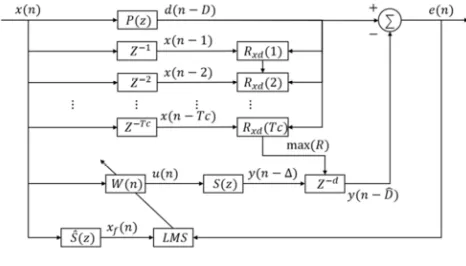
Figure 1. CTDE-FxLMS algorithm structure diagram.
In Figure 1, represents the system input, which is the noise signal collected by the reference microphone. represents the noise signal after the main channel transfer function , that is, the original noise signal input at the error sensor. represents the number of sampling points corresponding to the delay of the signal compared to . indicates that the input sequence is delayed by sampling intervals. represents the time two input sequences do correlation operation. represents the maximum range of the estimated delay of the system, which is determined according to the actual scenario. For the correlation matrix corresponding to different estimated delays at the same time, the maximum value is fed back to the delayer of the secondary path. is an adaptive filter for the noise cancellation part, using the least mean square error criterion. The parameters are adjusted by the system error received by the error sensor and the filter input signal obtained by estimation by the secondary channel . The filter output passes through the secondary channel to obtain a secondary output signal ∆ , where ∆ represents the number of sampling points corresponding to the secondary channel delay. The system output is obtained by the delayer , and is the estimation of the delay by the delay estimation part.
The addition of the delay estimation section and the delayer unit expand the tracking of the main channel delay by the system and must have the following conditions:
∆ (1)
That is, the main channel delay D, and the delay difference d between the main channel and the secondary channel are both positive values.
For the time delay estimation part, the correlation matrix between the delays from 1 to is calculated at the current time .
!" # $
%& $ %' $ %&%' (2)
(3)
By the nature of the autocorrelation function
| ++ , | - ++ 0 (4)
It can be seen that when , 0, ++ ∙ takes the maximum value, and , is the estimation of the system time delay at the current time.
012340 5" ++ , #6 (5)
Where arg is an operation taken from a variable.
The longer the sequence length L selected by the correlation operation, the more accurate the estimation result, but the amount of calculation will increase accordingly. Considering the refresh rate of the system delay estimation has certain requirements, the system design should be selected according to the actual situation.
The obtained estimated value is fed back to the delayer , and the delay point number d is calculated.
∆ (6) ∆ is the delay corresponding to the secondary channel sampling points, generally determined by the delay ADC, DAC and the processing time of the system brings.
For the noise cancellation part, the output of the filter
:; (7)
Where : ":< := :> ⋯ :@ = #; is the filter weight of length N at time n Coefficient vector,
" 1 2 ⋯ C $ 1 #; is the
input signal vector of length n with length N.
passes through the secondary channel to obtain the system output
∆ D ∗ (8)
Where D is the impulse response of , * represents the convolution operation, and ∆ is the cancellation waveform output by the secondary sound source.
The delayer delays the signal ∆ by
sampling intervals to obtain the signal .
The error signal represents the offset residual signal received by the error sensor
(9)
Calculate the filtered signal
D̂ ∗ (10)
Where D̂ is the impulse response of . Update the weight coefficient : of the filter
: $ 1 : G (11)
Where G is the step factor and its convergence range is as follows
0 H G H @I∆ J>
K (12)
Where N is the filter length and is the filter input signal power.
When the cancellation waveform y(n-D ̂) and the
original noise d(n-D) do not completely coincide in the time domain, the error e(n) tends to increase, thereby reducing the value of the step μ under the convergence condition.
Therefore, the convergence range of µ is updated to
0 H G H @I∆ +ILM J> +
KNO |P P| (13)
Where QD is the sampling frequency, is the slew rate of the sampled signal, specifically the upper limit of the change in the sampled value per second, and maxT T is the error of the delay estimate.
3. Experimental Simulation and Analysis
3.1. Experimental Basic Parameters
Experimentally simulate one channel selected in the spatial noise cancellation system, which is, one reference microphone, error sensor and secondary sound source. In the experiment, the sampling frequency is 11.025 kHz, the delay estimation uses 50 points for correlation operation, the noise cancellation part filter length is 21, the secondary channel delay is 10 sampling intervals, and the system estimates the maximum range of time delay Tc takes 100 sampling intervals. The noise selects the actual noise at the start of the motor and in the shifting state.
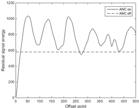
The effect of the number of output waveform offset points on the noise reduction effect is tested. The cancellation waveform is directly set to the inverse of the original noise. The result is shown in Figure 2.
Figure 2. The effect of signal offset points on the offset results.
meaningless. For the pulsed input signal, the upper limit of the number of offset points is more strict [20].
In order to ensure that the experiment achieves a more realistic simulation of the scene, two sets of experimental test algorithm performance are used. Experiment 1 does not change the relative position of the analog reference microphone and the error sensor, but there is a certain error in the measurement of the secondary channel delay. Experiment 2 simulates the situation where the reference microphone is offset due to environmental mechanical vibration. The delay between the reference microphone and the error sensor is considered here as a sinusoidal function that oscillates over time.
3.2. Main Channel Simulation of Fixed Length Delay
Set the true value of the main channel delay to 18 sampling intervals, and the delay of the a priori measurement is 17 sampling intervals. The measured values are only used for the calculation of the traditional FxLMS.
During the test operation, the system estimates the delay of the main channel. Considering the influence of the calculation amount, the system makes a delay estimation every 30 sampling intervals.
Figure 3. Comparison of estimated delay values under fixed time delay conditions.
Figure 4. Comparison of algorithm performance under real time delay fixed conditions.
The results of the operation are shown in Figure 3. It can be seen that the system estimates the delay of the main channel from 17 to 19 sampling intervals, and the values fluctuate around the true value.
The performance of the traditional FxLMS algorithm and the CTDE-FxLMS method is tested in this scenario. For the convenience of observation, the experimental results intercept 500 sampling intervals.
From the waveform point of view, the residual noise after the cancellation of the CTDE-FxLMS method is slightly lower than the traditional FxLMS algorithm.
Adding time delay estimation in the application scenario where the main channel delay is fixed enables the system to keep track of the true value of the delay, and has a good offset effect.
3.3. Main Channel Variable Length Delay Simulation
In order to simulate the phenomenon that the reference microphone or error sensor is accompanied by mechanical vibration in the scene, the true value of the delay is set to oscillate repeatedly with time, and the performance of the system and the delay tracking performance are tested.
The refresh rate of the delay estimate is the same as that of Experiment 1, which is 30 sample intervals. The main channel has a delay oscillation frequency of 40 Hz and an amplitude range of 20 to 40 sampling intervals. The traditional FxLMS algorithm uses a delay of 30 sampling intervals, and the true value of the delay is rounded up.
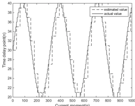
Figure 5. Comparison of estimated delay values under real delay variation.
The result of the operation is shown in Figure 5. It can be seen that the tracking of the main channel delay by the system basically conforms to the true value, and the error range is within 3 sampling intervals.
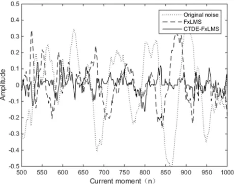
Figure 6 shows the performance comparison of the algorithm in a time-delayed environment.
Figure 6. Comparison of algorithm performance under real delay variation.
Table 1. Comparison of algorithm performance under different time delay environments.
Type of delay FxLMS CTDE-FxLMS
Constant time delay 28.65dB 24.24dB
Vibration time delay 16.70dB 8.83dB
3.4. Analysis of Experimental Results
The performance of the system under the condition that the main channel delay changes with time is significantly lower than that of the fixed delay condition. The FxLMS algorithm with delay estimation is 11.59dB higher than that of the non-added time under fixed time delay, and 14.13dB is improved in the oscillating environment, and the remaining energy is better for noise suppression. From the tracking performance of the delay estimation, the estimated value under the fixed delay condition has a slight fluctuation around the true value, and the estimated value under the oscillation delay condition has fluctuations of up to 4 sampling intervals around the true value. That is, the rate of change of the delay under the same refresh rate condition affects the accuracy of the delay estimation. The system with delay estimation under the same adaptive algorithm has better performance under experimental conditions.
4. Conclusion
In this paper, the application of correlation time delay estimation in ANC system is studied, and the influence of delay variation of main channel on system performance is expounded. The CTDE-FxLMS algorithm enables the system to estimate the delay of the main channel and the ability to track the delay of the main channel, achieving higher synchronization accuracy of the original noise and cancellation waveform in the time domain, thereby improving the noise cancellation effect. Through the simulation of two different scenarios, the improvement of system performance by adding delay is verified. In the representative application background, the rate and range of change of the main channel delay under environmental influence can be
measured in advance. In this way, the delay refresh rate that meets the system requirements is determined, and the system is stable and has low computational power requirements. This paper considers the passive influence of the surrounding environment on the main channel delay in the system. For the deployment of secondary sound sources, CTDE-FxLMS method is still applicable if a plurality of movable secondary sound sources are proposed for the noise reduction target of a specific optimized area in the future. At the same time, for scenarios where the main channel cannot acquire prior knowledge, the correlation time delay estimation can quickly converge to the true value, and the system adapts to the environment and environment changes in both the time domain and the frequency domain, so that the system has better adaptability.
References
[1] Zhang Yuexin, Liu Jian. Low frequency noise reduction in closed spaces based on multi-channel active noise control [J]. Science Technology and Engineering, 2018, 18 (35): 236-241. [2] Liu Enze, Yan Jikuan, Chen Duanshi. Research Overview and Development Trend of Noise Active Control System [J]. Noise and Vibration Control, 1999 (03): 2-6.
[3] Regis J. Serinko. Ergodic theorems arising in correlation dimension estimation [J]. Journal of Statistical Physics. 1996 (1-2).
[4] D. Dumont, X. Geets, M. Coevoet, E. Sterpin. EP-1669: Assessment of the clinical value of off-line adaptive strategies for tomotherapy treatments [J]. Radiotherapy and Oncology. [5] John Odell. Error estimation in stratigraphic correlation [J].
John Odell. Journal of the International Association for Mathematical Geology. 1975 (2).
[6] Constantinos N. Note on the estimation of the correlation function of neural spike trains [J]. Constantinos N. Christakos. Biological Cybernetics. 1984 (2).
[7] Su Yu, Lu Jianwei, Shao Haoran. Nonlinear active noise Control Based on Feedback System FxLMS [J]. The Journal of New Industrialization, 2018, 8 (03): 40-46.
[8] Li Nan, An Fengyan, Yang Feiran, Yang Jun. A Weighted-error-FxLMS Algorithm for active noise control headphone [J]. Journal of Applied Acoustics, 2018, 37 (03): 391-399.
[9] Zhang Shuai, Wang Yansong, Zhang Xinguang, Li Wenwu. Application of Variable Step-size Modified FxLMS Algorithm to Active Interior Noise Control for Vehicles [J]. Noise and Vibration Control, 2019, 39 (02): 64-69.
[10] Wang Guodong, Yang Peng. Active Noise Control System of Power Transformer Based on Adaptive Inverse Control [J]. Smart Power, 2016, 44 (09): 51-54+75.
[12] Ibrahem Shatnawi, Ping Yi, Ibrahim Khliefat. Automated intersection delay estimation using the input–output principle and turning movement data [J]. International Journal of Transportation Science and Technology. 2018 (2).
[13] Selahattin Ozcelik. Robust direct adaptive control for MIMO systems using Q-parameterization [J]. IFAC Proceedings Volumes. 2004 (12).
[14] Limin Zhang, Xiaojun Qiu. Causality study on a feedforward active noise control headset with different noise coming directions in free field [J]. Applied Acoustics, 2014, 80. [15] Ray Laura R, Solbeck Jason A, Streeter Alexander D, Collier
Robert D. Hybrid feedforward-feedback active noise reduction for hearing protection and communication. [J]. Acoustical Society of America. Journal, 2006, 120 (4). [16] Robert Hanus. Time delay estimation of random signals using
cross-correlation with Hilbert Transform [J]. Measurement, 2019, 146.
[17] Muhammad Tahir Akhtar, Wataru Mitsuhashi. Improving performance of FxLMS algorithm for active noise control of impulsive noise [J]. Journal of Sound and Vibration, 2009, 327 (3).
[18] Qiu Tianshuang, Wang Hongwei. Adaptive Time Delay Estimation in Time-varying Environments [J]. Journal of Ocean Technology, 1996 (02): 21-29.
[19] R. M. Fernández-Alcalá, J. Navarro-Moreno, J. C. Ruiz-Molina. Functional estimation incorporating prior correlation information [J]. Computational Statistics. 2007 (3).