Gini Support Vector Machine: Quadratic Entropy Based Robust Multi-Class Probability Regression

Gini Support Vector Machine: Quadratic Entropy Based Robust

Multi-Class Probability Regression

Shantanu Chakrabartty [email protected]

Department of Electrical and Computer Engineering Michigan State University

East Lansing, MI 48824, USA

Gert Cauwenberghs [email protected]

Division of Biological Sciences University of California San Diego La Jolla, CA 92093-0357, USA

Editor: Alex Smola

Abstract

Many classification tasks require estimation of output class probabilities for use as confidence scores or for inference integrated with other models. Probability estimates derived from large mar-gin classifiers such as support vector machines (SVMs) are often unreliable. We extend SVM large margin classification to GiniSVM maximum entropy multi-class probability regression. GiniSVM combines a quadratic (Gini-Simpson) entropy based agnostic model with a kernel based similar-ity model. A form of Huber loss in the GiniSVM primal formulation elucidates a connection to robust estimation, further corroborated by the impulsive noise filtering property of the reverse water-filling procedure to arrive at normalized classification margins. The GiniSVM normalized classification margins directly provide estimates of class conditional probabilities, approximating kernel logistic regression (KLR) but at reduced computational cost. As with other SVMs, GiniSVM produces a sparse kernel expansion and is trained by solving a quadratic program under linear con-straints. GiniSVM training is efficiently implemented by sequential minimum optimization or by growth transformation on probability functions. Results on synthetic and benchmark data, includ-ing speaker verification and face detection data, show improved classification performance and increased tolerance to imprecision over soft-margin SVM and KLR.

Keywords: support vector machines, large margin classifiers, kernel regression, probabilistic models, quadratic entropy, Gini index, growth transformation

1. Introduction

Support vector machines (SVMs) have gained much popularity in the machine learning community as versatile tools for classification and regression from sparse data (Boser et al., 1992; Vapnik, 1995; Burges, 1998; Sch ¨olkopf et al., 1998). The foundations of SVMs are rooted in statistical learning theory (Vapnik, 1995) with also connections to regularization theory (Girosi et al., 1995; Pontil and Verri, 1998a). The principle of structural risk minimization provides bounds on generalization performance which make SVMs well suited for applications with sparse training data (Joachims, 1997; Oren et al., 1997; Pontil and Verri, 1998b).

can also be used in combination with other probabilistic models such as hidden Markov models for inference across graphs. For instance text-independent speaker verification systems require normal-ized classifier scores to be integrated over several speech frames in an utterance (Auckenthaler et al., 2000) to arrive at global acceptance/rejection scores. Even though SVMs have been success-fully applied for the task of speaker verification (Schmidt and Gish, 1996; Gu and Thomas, 2001), the cumulative scores generated by SVMs are susceptible to corruption by impulse noise, which increases false acceptance rate.

Multi-class extensions to SVM classification have been formulated, based on ‘one vs. all’ (We-ston and Watkins, 1998; Crammer and Singer, 2000) or ‘one vs. one’ (Sch ¨olkopf et al., 1998; Di-etterich and Bakiri, 1995; Allewin et al., 2000; Hsu and Lin, 2002) methods. In its general setting multi-class SVMs generate unnormalized and biased estimates of class conditional probabilities (Platt, 1999a). Calibration and moderation methods have been proposed to arrive at class prob-ability estimates from the trained SVM classifier (Kwok, 1999; Platt, 1999a). For instance Platt (1999a) applied sigmoidal regression to the output of an SVM and showed a performance compa-rable to regularized maximum likelihood kernel methods (Jaakkola and Haussler, 1999; Zhu and Hastie, 2002). Vapnik has proposed a probability regression technique based on mixture of cosine functions (Vapnik, 1995), where the coefficients of the cosine expansion minimize a regularized function. A drawback of these methods is their difficulty in embedding other inference models like graphical models where re-estimation of SVM parameters can be naturally performed. Kernel logistic regression (KLR) (Jaakkola and Haussler, 1999) provides such a framework to estimate probabilities and can be easily embedded into graphical models with its parameters estimated us-ing an expectation-maximization (EM) like procedure (Jordan and Jacobs, 1994). However, one of the disadvantages of KLR is that the kernel expansion is non-sparse in the data making regression infeasible for large classification problems. A Bayesian learning framework using relevance de-termination on linear models more general than kernel regression (Tipping, 2001) produces a very sparse expansion but involves significant computation during training that does not scale well to very large data. Recently sparse Gaussian process based methods have been reported (Lawrence et al., 2003), that alleviate scalability problems of relevance determination through use of greedy optimization techniques.

The purpose of this paper is to describe a unifying framework for SVM based classification that directly produces probability scores. Previous work in this area used Shannon entropy in a large margin framework (Jebara, 2001) which led directly to KLR and hence inherited its potential disadvantages of non-sparsity. One of the important contributions of the paper is exploration of links between maximum entropy based learning techniques and large margin classifiers with exten-sions to quadratic based impurity functions. Within this framework the paper introduces the Gini Support Vector Machine (GiniSVM) (Chakrabartty and Cauwenberghs, 2002), a large margin clas-sifier based on a quadratic entropy formulation combined with kernel based quadratic distance. At the core of GiniSVM is a margin normalization procedure that moderates the output of the classi-fier. Training GiniSVM entails solving a quadratic programming problem analogous to soft-margin SVM. We also present algorithms for training GiniSVM classifiers with multiplicative updates, and by growth transformation on polynomial objective functions.

opti-mization (SMO) and a novel multiplicative update algorithm. Section 6 compares the performance of GiniSVM for benchmark UCI databases, a face detection and a text-independent speaker verifi-cation task. Section 7 provides concluding remarks with future directions.

2. Generalized Maximum Entropy Based Supervised Learning

In the framework of supervised learning, the learner is provided with a training set of feature vectors

T

⊂

X

:

T

={xi},i=1, ..,N drawn independently from a fixed distribution P(x),x∈

X

. The

formu-lation presented here assumes a countable set

X

even though it generalizes to uncountable sets. Also provided to the learner is a set of soft (or possibly hard) labels that represent conditional probability measures yik=P(Ck|xi) defined over a discrete set of classes Ck,k=1, ..,M. The labels therefore

are normalized and satisfy∑M_k=1yik=1. The aim of the learner is to choose a finite set of regression

functions P={Pk(x)},k=1, ..,M that accurately predict the true conditional probabilities P(Ck|x).

For this purpose the learner uses a distance metric DQ: RM×RM→R that embeds prior knowledge

about the topology of the feature space. Since the prior labels yikare available only for the training

set, the learner also defines an agnostic (non-informative) distance metric DI: RM×RM→R which

does not assume any knowledge of the training set. The embedded agnostic prior is consistent with maximum entropy principles (Jaynes, 1957; Pietra and Pietra, 1993) and enforces smoothness con-straints on the the function Pk(x)by avoiding solutions that over-fit to the training set. Estimating

the probability functions P={Pk(x)}entails a training procedure involving minimization of a joint

distance metric and is given by

min

P G(P) =minP [DQ(Y,P) +γDI(P,U)]. (1)

Here Y : R|T|×RM is a matrix of prior labels yik, i=1, ..,N, k=1, ..,M, and U denotes a uniform

distribution given by Uk(x) =1/M, ∀k=1, ..,M. γ>0 is a hyper-parameter that determines a

trade-off between the prior and agnostic distance metrics. Minimizing the cost function (1) leads to a solution P that is not only close to a prior distribution with respect to the distance metric DQ(., .)

but is also close to the non-informative (agnostic) uniform distribution U . In addition, the maximum entropy framework (Pietra and Pietra, 1993) allows to impose linear constraints on the optimization problem (1) based on cumulative statistics defined on the training set. One linear constraint equates the frequency of occurrence of a class k=1, ..,M under the distribution P to an equivalent measure under the prior distribution yik. This first constraint can be written to express equivalence between

average estimated probabilities and empirical frequencies for each class over the training set

N

∑

i=1

Pk(xi) = N

∑

i=1

yik, k=1, . . .M (2)

under the assumption that all features x∈

X

are equally likely. A second set of linear constraints expresses boundary and normalization conditions for valid probability distributions

Pk(x)≥0, k=1, . . .M, (3)

M

∑

k=1

Pk(xi) =1 (4)

D_Q(Y,P)

D_I(P,U) U

Y P

(a)

D_I(P,U) U

Y P

(b)

D_I(P,U) U

Y

P D_Q(Y,P)

(c)

Figure 1: Generalized framework for maximum entropy probability regression. (a): Solution P lies in the constraint space shown as a sphere such that the total distance to the distribution Y and U is minimized. (b): Solution forγ=0, where P coincides with Y . (c): Solution for

γ→∞, projecting U onto the constraint space.

Pictorially the solution to the optimization problem (1) is shown in Figure 1. For illustration purposes the linear constraints (2), (3) and (4) are represented by the shaded circle. The distance DQ(Y,P)determines the proximity of distribution P to a prior empirical distribution Y . DI(P,U)is a distance that defines an agnostic model when any prior knowledge about prior distribution is absent. This framework is similar to the maximum entropy approach (Jaynes, 1957; Pietra and Pietra, 1993; Jebara, 2001). The possible solutions to minimizing the cost function (1) with constraints (2)-(4) are shown in Figure 1 where the solution P lies within or at the boundary of the constraint space. Note that the constraint space also includes the prior distribution Y . Under non-degenerate conditions the agnostic U distribution will lie outside the constraint space. The value of the hyper-parameterγ>0 influences the location of the solution P with respect to the prior Y and agnostic U distributions. As we will see further below, the parameters also determine the sparsity and generalization perfor-mance of classifiers defined by parameters P. As shown in Figure 1, forγ=0, the solution is the prior distribution Y and thus over-fits to the training set. For the case whenγ→∞, the solution is equivalent to maximum entropy, which is the projection of U on the constraint space.

The solution to the optimization (1) is obtained by first order Karush-Kuhn-Tucker (KKT) con-ditions (Bertsekas, 1995) with respect to the probability functions P={Pk(x)}and is given by

γ∂DI(P,U)

∂Pk(x)

=−∂DQ(Y,P)

∂Pk(x)

+bk−z(x) +βk(x). (5)

Here bk represent Lagrange multipliers corresponding to frequency constraints (2), βk(x)≥0 are

Lagrange multipliers for the inequality constraints (3), and Lagrange multipliers z(x)correspond to the normalization constraint (4). For the sake of simplicity we will assume a form of DI(P,U)that

can be decomposed into independent, identically distributed (i.i.d.) components as

DI(P,U) = M

∑

k=1x

∑

∈T

Ψ(Pk(x),Uk(x)), (6)

whereΨ: R×R→R is a concave function. The first order condition (5) can be written as a Legendre transform (Rockefeller, 1970) with respect toΨ(.)as

Pk(x) =∇Ψ−1

1

γ

−∂DQ(Y,P)

∂Pk(x)

+bk−z(x) +βk(x)

where∇Ψ−1(.)denotes the Legendre transform with respect to Pk(x)for the bivariate functionΨ(.).

The Legendre transformation is commonly used in the dual formulation of support vector machines and other kernel machines (Vapnik, 1995; Sch ¨olkopf and Smola, 2001), and we refer to∇Ψ−1(.)as the dual potential function. Note that∇Ψ−1(.)is monotonic due to the concavity ofΨ(.).

Several choices exist for the prior distance metric DQ(., .). A popular metric is a quadratic distance extensively used in kernel methods (Sch ¨olkopf et al., 1998) and as covariance functions in Bayesian methods (Jordan and Jacobs, 1994). In its general form the quadratic distance between two conditional distributions ˆP={_Pˆ_{k(x)}and P={Pk(x)}is given by}

DQ(_Pˆ_{,P) =}C 2

M

∑

k=1x,

∑

v∈T

K(x,v)_Pˆ_{k(x)−Pk(x)P}ˆ_{k(v)−Pk(v). (8)}

Here K : RM×RM →R represents a symmetric, positive definite kernel satisfying the Mercer’s criterion,1 such as a Gaussian radial basis function or a polynomial spline (Sch ¨olkopf et al., 1998; Wahba, 1998). The distance DQ(., .) embeds prior knowledge induced by the kernel K(x,v) and therefore quantifies a topology of a metric space for points x,v∈

X

.

For the quadratic form DQ(., .)given by Equation (8) the first order conditions (7) can be written

as

Pk(x) =∇Ψ−1

1

γ[fk(x)−z(x) +βk(x)]

(9)

where

fk(x) = N

∑

i=1

λi

kK(xi,x) +bk

with inference parameters

λi

k=C[yik−Pk(xi)].

The Lagrange parameter functionβk(x)in Equation (9) needs to ensure that the probability scores

Pk(x)≥0 ∀x∈

X

according to (3), and the Lagrange parameter function z(x) needs to ensure

normalized probabilities∑M_k=1Pk(x) =1 according to (4). The set of inference parameters Λ={λi

k},i=1, ..,N, k=1, ..,M is obtained by solving (1)

over the training set

T

. Expressing the general form (6) for the agnostic distance DI(P,U)and the

quadratic distance (8) for the prior distance DQ(Y,P)in terms of the inference parametersλi_kin the cost function (1) leads to a dual formulation Hd

Hd= M

∑

k=1

"

1 2C

N

∑

i=1

N

∑

j=1

λi

kQi jλ_kj+γ N

∑

i=1

Ψ(yik−λik/C) #

(10)

where Qi j=K(xi,xj)denote elements of the kernel matrix Q. Like the primal (1), minimization of

the dual Hdis subject to linear constraints (2)-(4) rewritten in terms of the inference parameters as

M

∑

k=1

λi

k = 0, i=1, . . .N,

N

∑

i=1

λi

k = 0, k=1, . . .M, (11)

λi

k ≤ Cyik.

3. Kernel Logistic Regression

For a frame of reference in the comparison between different formulations of cost functions, the optimization framework given by the dual (10) subject to constraints (11) is first applied to kernel logistic regression (KLR) (Jaakkola and Haussler, 1999), with agnostic distance

DI(P,U) = M

∑

k=1x

∑

∈T

Pk(x)logPk(x) Uik

= M

∑

k=1x

∑

∈T

Pk(x)log Pk(x) +cst (12)

derived from the Kullback-Leibler (KL) divergenceΨKL(P,U) =P log(P/U)for a uniform agnostic distribution Uik≡1/M. The constant term cst=N log M in (12) drops in the minimization and is

subsequently ignored. The probability function according to (9) is then given by

Pk(x) =exp

1

γ[fk(x)−z(x) +βk(x)]

. (13)

By property of exp(.), Pk(x)≥0 ∀x∈

X

, and so the Lagrange multiplierβk(x)in (13) is arbitrary

and can be eliminated, βk(x)≡0. The other Lagrange multiplier z(x) in (13) is determined by

expressing the normalization condition∑M_k=1Pk(x) =1 which leads to a logistic model Pk(x) =exp

1

γfk(x))/ M

∑

p=1

exp(1

γfp(x) !

. (14)

Substituting the KL distanceΨKL(., .)forΨ(., .)in the general form (10) directly leads to the dual

cost function

He= M

∑

k=1

"

1 2C

N

∑

i=1

N

∑

j=1

λi

kQi jλ_kj+γ N

∑

i=1

(yik−λik/C)log(yik−λik/C) #

(15)

subject to the dual constraints (11).

3.1 KLR Primal Reformulation

The dual (15) derived from the general maximum entropy form (1) is identical to the dual formu-lation of another, closely related primal cost function for kernel logistic regression as formulated in Jaakkola and Haussler (1999). The purpose of this section is to establish the equivalence with a connection to large margin kernel machines and their interpretation in feature space (Sch ¨olkopf and Smola, 2001).

Expressing the kernel function K(x,v) =Φ(x)·Φ(v)as an inner-product in a transformed fea-ture spaceΦ(.), the decision functions fk(x)are linked to a set of M hyperplanes

fk(x) = N

∑

i=1

λi

k K(xi,x) +bk (16)

= N

∑

i=1

λi

k Φ(xi)·Φ(x) +bk (17)

where wk=∑Ni=1λikΦ(xi)represent the parameters of the hyperplanes. The following proposition

links the kernel logistic regression dual (15) with its equivalent primal formulation (Jaakkola and Haussler, 1999).

Proposition I: The kernel logistic regression objective function (15) is the dual derived from a primal objective function with regularized loss function

Le = M

∑

k=1

1 2|wk|

2_+C

∑

N

i=1

M

∑

k=1

yiklog

yik

Pk(xi)

=

∑

k=1 1 2|wk|

2_−C

∑

N

i=1

[ M

∑

k=1

yikfk(xi)−log(ef1(xi)+...+efM(xi))]. (18)

where additional constant terms in (18) have been ignored and a unity value forγhas been assumed in the probability model (14). The proof of the proposition is provided in Appendix A.

The primal uses the Kullback-Leibler (KL) divergenceΨKL(P,U) =P log(P/U)between

distri-butions yikand Pk(xi)as loss function in the regularized form (18) (Wahba, 1998; Zhu and Hastie,

2002). One of the disadvantages of the kernel logistic dual is that the KL divergence distance metric strongly penalizes solutions far away from the agnostic distribution U , leading to a non-sparse ker-nel expansion. A sparser kerker-nel expansion is obtained in soft-margin support vector machines for classification. A Gini form of entropy as agnostic distance metric provides the connection between support vector machines and probability regression, studied next.

4. GiniSVM and Margin Normalization

Instead of KL divergence, a natural choice for an agnostic distance metric DI is a quadratic form

of entropy similar to the quadratic form of the prior distance metric DQ. A Gini quadratic form of

entropy, or impurity function, has been used extensively in natural language processing for growing decision trees (Breiman et al., 1984). The Gini quadratic entropy forms the basis of the Gini-support vector machine (GiniSVM) for probability regression (Chakrabartty and Cauwenberghs, 2002).

The Gini quadratic form of entropyΨGini(P,U) = 1₂(P−U)2_{with uniform agnostic distribution} Uik≡1/M leads to an agnostic distance metric

DI(P,U) =

1 2

M

∑

k=1x

∑

∈T

(Pk(x)−Uik)2

= 1

2

M

∑

k=1x

∑

∈T

Pk(x)2+cst

where the constant term cst=−N/2M drops in the minimization. Substituting the Gini distance

ΨGini(., .)forΨ(., .)in the general form (10) leads to the dual GiniSVM cost function

Hg= M

∑

k=1

"

1 2C

N

∑

i=1

N

∑

j=1

λi

kQi jλ_kj+γ

2

N

∑

i=1

(yik−λik/C)2 #

(19)

under constraints (11).

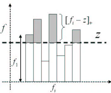
Figure 2: Illustration of reverse water-filling procedure. The level z is adjusted as to maintain the net fiin excess of z (shaded area) atγ.

to zero by the inequality constraints in (11) corresponding to a majority of labels for which yik=0.

Even sparser kernel expansions could be obtained with soft-margin support vector machines for classification, owing to its slightly different quadratic cost function under linear constraints which further favors sparsity. More significantly, GiniSVM produces conditional probability estimates that are based on maximum entropy (1). The probability estimates themselves could be sparse, with Pk(x) =0 for a number of classes k depending onγand x, as we show next.

4.1 Margin Normalization and Reverse Waterfilling

The quadratic entropy form ofΨGini(., .)leads to a linear Legendre transform∇Ψ−1(.)and thus a linear, rather than exponential, form of the conditional probability estimates Pk(x) =1/γ/[fk(x)−

z(x) +βk(x)],k=1, ..,M. To ensure positive probabilities according to constraints (3), the Lagrange

parametersβk(x)produce rectified linear probability estimates

Pk(x) =

1

γ[fk(x)−z(x)]+ (20)

where[x]+=max(x,0) denotes a hinge function. The remaining Lagrange parameter z(x)is

de-termined through a subtractive normalization procedure which solves for the normalization con-straint (4)

M

∑

k=1

[fk(x)−z(x)]+=γ. (21)

The conditions (20) and (21) are jointly satisfied by applying a reverse water-filling algorithm com-monly found in communication systems (Cover and Thomas, 1991), listed in Algorithm 1 and illus-trated in Figure 2. The algorithm recursively computes the normalization factor z(x)such that the net balance of class confidence levels fk(x)in excess of z(x)equalsγ.

We refer to the procedure solving for z(x) given confidence scores fk(x) in (21) as margin

Algorithm 1 Reverse water-filling procedure to compute normalization parameter z Require: Set of confidence values{fk(x)},k=1, ..,M.

Ensure: z=0,N=1,T=0 a=max{fk(x)}

{s} ← {fk(x)} − {a}

while T <γ & N<M do b=max{s}

T ←T+N(a−b)

a←b

{s} ← {s} − {b} N←N+1

end while

z←b+N(γ−T)

normalization (14) of probabilities in kernel logistic regression, the subtractive margin normal-ization (20)-(21) in GiniSVM offers several distinct properties in connection with margin based classifiers:

Monotonicity: Let fk(x),k=1, ..,M a set of GiniSVM decision functions satisfying the reverse

water-filling conditions∑M_k=1[fk(x)−z1(x)]+=γ1 and ∑Mk=1[fk(x)−z2(x)]+ =γ2. Ifγ1≥γ2>0, then z1(x)≤z2(x).

Proof: The two reverse water-filling conditions lead to

M

∑

k=1

([fk(x)−z1(x)]+−[fk(x)−z2(x)]+) =γ1−γ2>0.

The convexity of the hinge function[a−b]+≥[a]+−[b]+; a,b∈

R

leads to

[z2(x)−z1(x)]+≥(γ1−γ2)/M>0 which is equivalent to z2(x)>z1(x).

Sparsity: The effect of rectification (20) in the subtractive normalization (21) is to produce a number 0≤m<M of classes k1, . . .km∈ {1, . . .M}with zero probabilities Pkj(z) =0, for which

the normalization level z(x) exceeds the confidence level fkj(x). As a direct consequence of the

monotonicity property, decreasing the margin parameter γleads to a larger number m of classes with zero probabilities. Therefore the margin parameterγ directly controls the sparsity m of the probability estimates, assigning the probability mass to a smaller fraction of more confident classes with larger fk(x)asγis decreased. Besides the dependence on γ, the number of zero probability

classes m depends on the actual values of fk(x), and hence on the inputs x.

Margin: In the limitγ→0, the normalization factor z(x)→maxkfk(x). Thus asγ→0, margin

normalization acts as ‘winner-take-all’, m→M−1, and strongly favors the highest class score. Based on this principle a multi-class probability margin can be defined based on the multi-class decision functions fk(x)as fk(x) =z(x) +γ. The effect of the hyper-parameter γcan be seen on

−0.5 0 0.5 1 1.5 0

0.5 1 1.5

x 1

x 2

(a)

−0.5 0 0.5 1 1.5

0 0.5 1 1.5

x 1

x 2

(b)

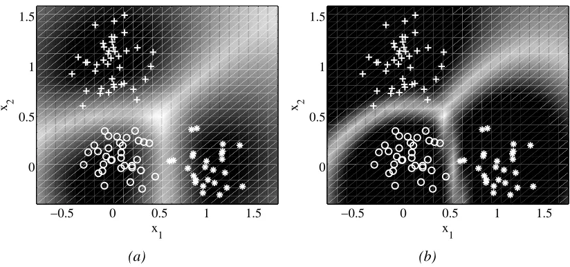
Figure 3: Equal probability contour plots for a three-class problem with the GiniSVM solution obtained for (a)γ=8 and (b)γ=0.08.

by ’white’ region). Similar to soft-margin SVM the location of the margin determines the sparsity of the GiniSVM solution. This is illustrated in Figure 3(a)-(b). Shades in the figure represent equal probability contours, and the extent of ’white’ regions around the decision boundaries illustrates the margin of separation. It can be seen from Figure 3(a)-(b) that reduction in γhas the effect of increasing the size of the margin, and thereby controls the sparsity of the GiniSVM solution.

Robustness: The subtractive margin normalization (20) and (21) is inherently robust to impulsive noise, since components fk(z) in the kernel expansion smaller than a threshold z(x) (at most a

marginγbelow the largest value) do not contribute to the output.2 In a physical implementation of margin decoding, adjusting the levelγaccording to the noise floor leads to significant improvements in decoding performance (Chakrabartty and Cauwenberghs, 2004). The robustness properties of GiniSVM in relation to the thresholdγare further analyzed in Section 4.4.

4.2 GiniSVM Primal Reformulation

In this section we derive an equivalent primal reformulation of the GiniSVM dual (19), analogous to the derivation in Section 3.1. As for the multi-class logistic primal (18), decision functions for classes k=1, ..,M are expressed in terms of a set of M hyperplanes fk(x) =wk˙Φ(x) +bk. Given

a set of training vectors xi∈

R

D,i=1, ..,N and its corresponding prior probability distributions

yik∈

R

: yik≥0;∑Mk=1yik=1, GiniSVM in its primal reformulation of minimizes a regularization

factor proportional to the L2 norm of the weight vectors wk,k=1, ..,M and a quadratic loss function

2. The subtractive normalization is insensitive only to negative impulsive noise in fk(z). Typically, a choice of kernel

lgaccording to

Lg=

1 2

M

∑

k=1

|wk|2+ N

∑

i=1

M

∑

k=1

lg(wk,bk,zi) (22)

with loss function lg(xi)for each training vector xigiven by

lg(xi) =

γC 2

yik−

1

γ[fk(xi)−zi]+

2

,

and where zi, i=1, . . .N are free parameters entering the minimization of Lg, along with the

hyper-plane parameters wk and bk, k=1, . . .M.

Proposition II: Denote the solution to the minimization of Lgas

(w∗_k,b∗_k,z∗_i) =argmin_wk,bk,ziLg,

then

1. Pk(xi) = 1_γ[f_k∗(xi)−z∗i]+ with fk∗(xi) = w∗k·xi+b∗k for a given data xi is a valid

condi-tional probability measure over classes k ∈1, ..,M, where zi performs the normalization

∑M

k=1Pk(xi) =1.

2. The dual cost function corresponding to the primal cost function (22) is the GiniSVM dual (19).

The proof of the proposition is given in Appendix B.

4.3 Binary GiniSVM and Quadratic SVM

In one case of interest the multi-class GiniSVM solution simplifies to a binary class problem, where the learner is provided with binary labels yi∈ {−1,+1}representing class membership of a feature

vector xi∈

T

. Binary GiniSVM entails regression of a single probability P+1(x) =1−P−1(x)as a function of a single margin variable f(x) = 1

2(f+1(x)−f−1(x)). Elimination of the normalization parameter z from the binary version of (20) constrained by (21) yields

P+1(x) =

f(x)

γ +

1 2

1 0

(23)

where[.]1

0denotes a limiter function confining the probability to the [0,1] interval,[a]10= [a]+−[a− 1]+. With the kernel expansion of f(x)expressed in reduced form3

f(x) = N

∑

i=1

λi_y

iK(xi,x) +b, (24)

the GiniSVM dual objective function (19) and linear constraints (11) reduce to

Hb=min λi

1 C

" N

∑

i=1

N

∑

j=1

λi_λj_y

iyjK(xi,xj)− N

∑

i=1

G(λi₎ #

(25)

3. This choice of kernel expansion is consistent with binary soft-margin SVM and binary KLR, with identical dual

ψ-1

0

γ

C

C

λ

i

M

l_g

1

y_i f(x_i)

4

γC

2

γ

2

γ

2

γ

2

γ

2

(y_i f(x_i)) y_i f(x_i)

P₊₁

P₊₁ =

0 _G

(

λ

i

) =

ψ

(P

+1

)

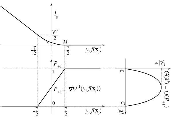
Figure 4: Graphical illustration of the relation between binary GiniSVM dual potential function G, inference parametersλi, probability estimates Pi, and primal loss function lg.

under constraints

M

∑

i=1

λi_y i=0,

0≤λi≤C

with dual potential function

G(λ) =γCλ C(1−

λ

C). (26)

The derivation is given in Appendix C.

Figure 4 graphically illustrates the relationship between the binary GiniSVM dual potential function G, inference parametersλi, probability estimates Pi, and primal reformulation loss function

lg. The dual potential is linked to the probability estimate through the Legendre transform∇Ψ−1(.)

as described by Equations (5)-(7). Since the dual potential function is symmetricΨ(P+1) =Ψ(1− P+1) =Ψ(P−1), it follows that the Legendre transform ∇Ψ−1(.) is antisymmetric and hence the probability estimates are centered around the discrimination boundary, P+1(f(x)) =1−P+1(−f(x)) consistent with the functional form (23). Symmetry in the dual potential function thus leads to unbiased probability estimates that are centered around the discrimination boundary, P+1=P−1= 1/2 for f(x) =0.

The Legendre transform also links the dual potential function to the primal reformulation cost function. Note the relationship between the parameter γscaling the dual potential function, and the location of the margin in the loss function and probability estimate indicated by M in Figure 4. Hence the parameterγcan be seen both to control the strength of the agnostic metric DI, and to

−5 0 5 0

1 2 3 4 5 6

Margin y f(x)

Loss

l

Logit

Gini

SVM

(a)

0 0.2 0.4 0.6 0.8 1

0 0.1 0.2 0.3 0.4 0.5 0.6 0.7 0.8 0.9 1

Inference Parameter λ

P

o

tent

i

a

l

Fu

nct

io

n

G

Logit Gini SVM

(b)

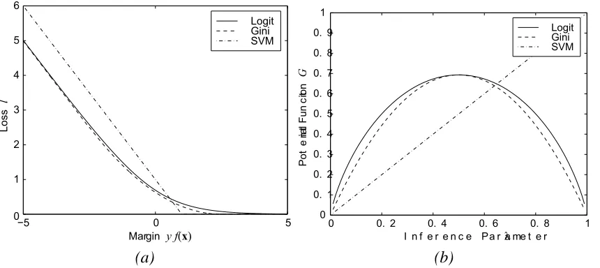
Figure 5: Primal and dual formulation of logistic regression, GiniSVM regression and soft-margin SVM classification. (a): Loss function in the primal formulation. (b): Potential function in the dual formulation. The GiniSVM loss function and potential function closely ap-proximate those for logistic regression, while offering the sparseness of soft-margin SVM classification. C=1, andγ=8 log 2 for GiniSVM andγ=1 for logistic regression.

A direct comparison can be made between the binary GiniSVM formulation and other binary classifiers by inspecting differences in their potential functions G(u), shown in Figure 5(b). The GiniSVM potential function is symmetric around the center of the agnostic, uniform distribution U=1/2 where it reaches its maximum. The center corresponds to the origin of the margin variable yif(xi)in Figure 5(a) which represents the separating hyperplane. Figure 5(b) also shows the binary

KLR dual potential function given by Shannon’s binary entropy (Jaakkola and Haussler, 1999)

G(λ) =γC

_λ

Clog(

λ

C) + (1−

λ

C)log(1−

λ

C)

.

Like GiniSVM, the binary KLR dual potential function is symmetric with respect to the separating hyperplane in Figure 5(a), and hence also produces unbiased estimates of conditional probabilities. In contrast, the soft-margin SVM potential function G(λ) =λis asymmetric with respect to the separating hyperplane and produces biased or skewed conditional probability estimates. The binary GiniSVM dual bears similarity to the quadratic SVM dual (Sch ¨olkopf et al., 1998), but the quadratic SVM lacks the symmetry of the potential function around the separating hyperplane.

4.4 Relation to Robust Estimation and Logistic Regression

The GiniSVM dual (19) relates to the kernel logistic regression dual (15) through a lower-bound on Shannon entropy. Using the inequality log x≤x−1,x≥0, the Shannon entropy term Ge(P) =

−∑M

k=1Pklog Pkis everywhere larger than the Gini entropy Ge(P)≥1−∑ikPik2. This is illustrated in

Figure 5(b) which compares the potential functions for KLR and GiniSVM in the binary case. Both expressions of entropy reach their maximum for a uniform distribution, P= 1

that the solution obtained by minimizing the GiniSVM dual Hgin Equation (19) is an over-estimate

of the solution obtained by minimizing kernel logistic dual He given by Equation (15). In fact we

found that initial iterations decreasing the cost Hgalso resulted in a decrease of He with deviations

evident only near convergence. Thus the GiniSVM dual Hg can also be used for approximately

solving the kernel logistic dual He.

The loss function corresponding to binary GiniSVM can be visualized through Figure 5(a) and compared with other primals. For binary-class GiniSVM, ‘margin’ is visualized as the extent over which data points are asymptotically normally distributed. Using the notation for asymptotic nor-mality in Huber (1964), the distribution of distance z from one side of the margin for data of one class4is modeled by

F(z) = (1−ε)

N

(z,σ) +ε

H

(z)

where

N

(.,σ)represents a normal distribution with zero mean and standard deviation σ,

H

(.)is the unknown symmetrical contaminating distribution, and 0≤ε≤1.

H

(.) could, for instance, represent impulsive noise contributing outliers to the distribution.

Huber (1964) showed that for this general form of F(z) the most robust estimator achieving minimum asymptotic variance minimizes the following loss function:

g(z) = (

1 2

z2

σ2 ; |z| ≤kσ

k|_σz|−1 2σk

2 _{; |z|>kσ} (27)

where in general the parameter k depends onε. For GiniSVM, the distribution F(z)for each class is assumed one-sided (z≤0). In particular, the Huber loss function g(z) in (27) reduces to the binary GiniSVM loss function lg(y f(x)), shown in Figure 4, for z≤0 with z=y f(x)−γ/2, kσ=γ, and k/σ=C. Therefore the parameterγin GiniSVM can be interpreted as a noise margin in the Huber formulation, consistent with its interpretation as noise threshold in the reverse water-filling procedure for margin normalization. As with soft-margin SVM, points that lie beyond the margin (z>0) are assumed correctly classified, and do not enter the loss function (g(z)≡0). The binary GiniSVM loss function is a special case of Huber loss used in quadratic SVMs (Sch ¨olkopf et al., 1998) which directly generates normalized scores from the margin variable f(x).

5. GiniSVM Training Algorithm

GiniSVM training entails solving a quadratic optimization problem for which several standard pack-ages and algorithms are available (Platt, 1999b; Cauwenberghs and Poggio, 2001; Osuna et al., 1997). Most of these methods exploit the underlying structure in the classification problem to in-corporate heuristics that considerably speed up the convergence of the training algorithm. In this section we describe two algorithms for optimizing GiniSVM dual function (19). The first algorithm uses a decomposition algorithm called sequential minimal optimization. The second algorithm uses the polynomial nature of the dual resulting into a novel multiplicative update algorithm based on growth transformation on probabilities.

5.1 Sequential Minimal Optimization

Sequential minimal optimization (Platt, 1999b) is an extreme case of a decomposition based quadratic program solver, where a smallest set of inference parameters is chosen each iteration, and optimized subject to the linear constraints. The advantage of SMO is that it can be efficiently implemented without resorting to QP packages, and it scales to very large data sets. In the case of the GiniSVM dual function (19), at least four inference parameters need to be chosen to satisfy two sets of equality constraints (11). A randomized version of SMO algorithm is described in Algorithm 2.

Algorithm 2 Randomized SMO algorithm

Require: Training data xi,i=1, ..,N and labels yik,i=1, ..,N,k=1, ..,M Ensure: Letλi_k=0 for i=1, ..,N,k=1, ..,M.

repeat

•Randomly choose a set of four inference parametersλ1₁,λ1

2,λ21andλ22. •Updateλ1₁,λ1

2,λ21andλ22such that the dual (19) is minimized subject to constraints (11).

until convergence

The derivation of the SMO update rule based on the choice of inference parameters is given in Appendix D. Instead of random selection of working sets of inference parameters, heuristics based on the structure of the classification problem can be used to speed up convergence (Platt, 1999b; Keerthi et al., 2001). Standard QP algorithmic methods for SVM training such as caching and shrinking besides chunking (Joachims, 1998) can be applied to further speed up convergence of SMO training.

5.2 Growth Transformation on Generalized Polynomial Dual

In lieu of the inference parameters defined asλi_k=C[yik−Pk(xi)], the GiniSVM dual in (19) can be

expressed in terms of probabilities Pik=Pk(xi)as

H=C

2

M

∑

k=1

"_N

∑

i=1

N

∑

j=1

Qi j[yik−Pik]

yjk−Pjk

+γ

2

N

∑

i=1

P_ik2

#

(28)

with linearity constraints (3) and (4) to ensure valid probabilities, Pik≥0,∀i,k and∑Mk=1Pik=1,∀i.

For the remainder of the derivation the additional equality constraint (2) corresponding to the bias term b will be relaxed. Artifacts due to absence of the bias b can reduced by properly pre-processing and centering the training data or by incorporating an additional input dimension in the kernel func-tion. The optimization function (28) is a non-homogeneous polynomial with normalized probability variables Pik,∀i and with possibly negative coefficients. We can directly apply results from Baum

and Sell (1968) and Gopalakrishnan et al. (1991) to optimize the dual (28).

Theorem 2 (Gopalakrishnan et al.) Let H({Pik}) a polynomial of degree d in variables Pik

in the domain D : Pik≥0,∑q_k=i ₁Pik=1,i=1, ..,N,k=1, ..,qisuch that∑q_ki₌₁Pik_∂P∂H_ik(Pik)/6=0 ∀i.

Define an iterative map according to the following recursion

b

Pik←

Pik(_∂∂H_P

ik(Pik) +Γ)

∑qi

k=1Pik(∂P∂Hik(Pik) +Γ)

−4 −3 −2 −1 0 1 2 3 4 −0.2

0 0.2 0.4 0.6 0.8 1

X

P 1

( X

)

Gini KLR SVM Bayes

Figure 6: Probability estimates generated by GiniSVM, KLR and a calibrated soft-margin SVM for one-dimensional synthetic training data.

whereΓ≥Sd(N+1)d−1 _{with S being the smallest coefficient of the polynomial H({P}

ik}). Then

{Pbik} ∈D and H({Pbik})>H({Pik}).

The result can be applied for minimizing the polynomial dual corresponding to Equation (29). Let P_ik0 =1/M the initial value of the probability distribution for all i,k, and assume the kernel matrix be bounded such that|Qi j| ≤Qmax,∀i,j. Also, let Pikmthe value of the probability distribution

at mthiteration then

P_ikm+1←P_ikmδm_ik/ M

∑

k=1

P_ikmδm_ik

where

δm ik=C

N

∑

j=1

Qi j[Pikm−yik] +γPikm+Γ

andΓ=C (N+1) Qmax. At each update the cost function (28) decreases, and the procedure is

repeated till convergence. Due to the multiplicative nature of the update some distribution variables Pikcan never reach unity or zero; however, in practice it approaches the limits within given margins

of precision similar to other implementations of SVM training algorithms. As with other SVM optimization techniques, the speed of large margin growth transformation can be enhanced by using caching and shrinking (Joachims, 1998), as values of the distribution Pikclose to unity or zero almost

0 0.2 0.4 0.6 0.8 1 0

0.1 0.2 0.3 0.4 0.5 0.6 0.7 0.8 0.9 1

P(y| X) Py

( X

)

(a)

0 0.2 0.4 0.6 0.8 1 0

0.1 0.2 0.3 0.4 0.5 0.6 0.7 0.8 0.9 1

P(y| X) Py

( X

)

(b)

Figure 7: Comparison between conditional Bayes probability estimates and scores generated by GiniSVM for 10-dimensional synthetic data with (a)γ=0.8 and (b)γ=0.08.

6. Experiments and Results

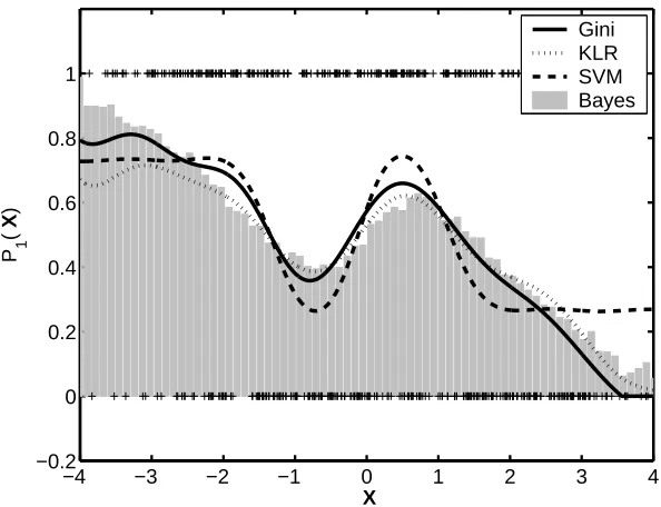
The first set of experiments were designed to characterize the probability scores generated by GiniSVM for synthetic data. Figure 6 compares the scores generated by GiniSVM, KLR and soft-margin SVM for a synthetic binary classification problem. The one dimensional training data corresponding to two classes were generated using a bimodal Gaussian distribution. A histogram generated by data points randomly sampling the distribution is shown in Figure 6 and the locations of 500 data points used for training are denoted by ‘+’ along y=1 and y=0. For the soft-margin SVM the scores were normalized using Platt’s calibration procedure (Platt, 1999a). The Figure 6 shows that the scores generated by KLR, GiniSVM and calibrated soft-margin SVM are similar and approximate the sampled distribution which approximates the Bayesian optimum solution. It can be seen that calibrated soft-margin SVM scores do not approximate the true conditional distribution at the boundary of the distribution and would require additional parameterization for producing better estimates.

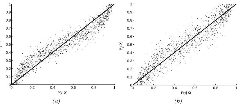
Figures 7(b) and (c) compare GiniSVM scores with sampled conditional scores (Bayes esti-mates) for synthetic data in 10 dimensions. The data were generated from a multi-variate Gaussian distribution, out of which 100 data points were chosen for training. Figures 7(a) and (b) demon-strate a monotonic relationship between GiniSVM scores and Bayes estimate of class conditional probabilities. The sigmoidal relationship trend shown in the scatter plot 7(a) forγ=0.8 is attributed to linear approximation of the logistic model (14) by subtractive normalization model (20).

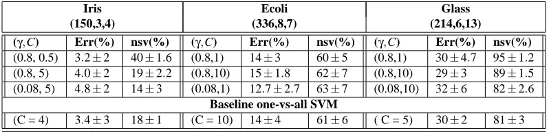
The performance of GiniSVM based classifier was evaluated on three benchmark UCI databases

and compared with a baseline one-vs-all soft-margin SVM classification method

Iris Ecoli Glass (150,3,4) (336,8,7) (214,6,13)

(γ,C) Err(%) nsv(%) (γ,C) Err(%) nsv(%) (γ,C) Err(%) nsv(%)

(0.8, 0.5) 3.2±2 40±1.6 (0.8,1) 14±3 60±5 (0.8,1) 30±4.7 95±1.2

(0.8, 5) 4.0±2 19±2.2 (0.8,10) 15±1.8 62±7 (0.8,10) 29±3 89±1.5

(0.08, 5) 4.8±2 14±3 (0.08,1) 12.7±2.7 63±7 (0.08,10) 32±6 82±2.6

Baseline one-vs-all SVM

(C = 4) 3.4±3 18±1 (C = 10) 14±4 61±6 ( C = 5) 30±2 81±3

Table 1: Performance of GiniSVM classifier on UCI database.

kernel K(x,y) =exp(− 1

2σ2(x−y)T(x−y))was chosen for all experiments. The kernel parameter

σand the regularization parameter C were chosen based on the performance of the baseline SVM

on a held-out set. The same kernel parameter was used for training GiniSVM classifiers. Table 1 shows the error rate (indicated by Err) and the number of support/error vectors (indicated by nsv) obtained for different sets of hyper-parametersγand C. The results indicate that the classification performance of the GiniSVM based system is comparable to the baseline one-vs-all SVM system. The results also illustrate the effect ofγon the sparseness of the solution which increases asγ→0, as explained using the generalized dual framework in Section 4.

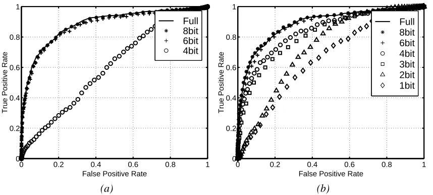
6.1 Face Detection and Effects of Parameter Mismatch

The advantage of GiniSVM over conventional soft-margin SVM is demonstrated by performing sensitivity analysis on the kernel expansion at completion of training. For this experiment a face detection task was chosen. The classifiers were trained using the face detection database available through CBCL at MIT (Alvira and Rifkin, 2001) and their performance was evaluated on the stan-dard CMU-MIT test set (Rowley et al., 1998). Training of the classifier was performed by utilizing floating point precision arithmetic, whereas evaluation was performed after quantizing the support vectors and inference parameters to 8,6 and 4 bits, and adding 1 LSB of uniform random noise. For this experiment the parameter C was determined by optimizing the performance of the classifier on a held-out data set. Receiver operating characteristics (ROC) were obtained by evaluating the performance of the mismatched classifier on the test set. Figure 8 compares ROC curves for the classifier trained with soft-margin SVM, vs. another trained identically with GiniSVM for a 2nd

order polynomial kernel. The results indicate that GiniSVM solution is more robust to mismatch and precision errors in the inference parameters. In fact for this data set, the GiniSVM solution quantized to 1 bit is more robust than an equivalent soft-margin SVM solution quantized to 4 bits.

6.2 Speaker Verification Experiments

0 0.2 0.4 0.6 0.8 1 0

0.2 0.4 0.6 0.8 1

False Positive Rate

True Positive Rate

Full 8bit 6bit 4bit

(a)

0 0.2 0.4 0.6 0.8 1

0 0.2 0.4 0.6 0.8 1

False Positive Rate

True Positive Rate

Full 8bit 6bit 4bit 3bit 2bit 1bit

(b)

Figure 8: ROC obtained for a face detection system trained with (a): soft-margin SVM and (b): GiniSVM training algorithm, for a 2ndorder polynomial kernel.

contiguous 25ms speech samples were extracted and Mel-frequency cepstral coefficient (MFCC) features were extracted. The MFCC feature extraction procedure has been extensively studied in the literature and details can be found in Rabiner and Juang (1993). A 39-dimensional feature vec-tor was formed by concatenating the total energy in the speech frame, along with the∆and∆−∆ MFCC coefficients.

For training, 100 speakers (speaker ID: 101-200) were chosen from the YOHO database and MFCC features were extracted for all speech frames corresponding to each speaker. To reduce the total number of training points, a K-means clustering was performed for each speaker to obtain 1000 cluster points for the correct speaker, and 100 cluster points for each imposter speaker. For each speaker (101-200), this procedure was repeated to obtain a training set of 10,900 MFCC vectors.

Classifiers specific to each speaker were trained using a GiniSVM toolkit

(http://bach.ece.jhu.edu/svm/ginisvm). For testing utterances corresponding to 100 speakers were chosen from the YOHO test set. Confidence scores generated by GiniSVM for each speech frame were integrated over the duration of the utterance to obtain the final cumulative score. Thus each speech frame is treated to be independent and their scores are integrated together without taking into account any time-based correlations.

0 0.01 0.02 0.03 0.04 0.05 0.06 0.84

0.86 0.88 0.9 0.92 0.94 0.96 0.98 1

False Acceptance Rate

True Acceptance Rate

KLR

SVM

Gini

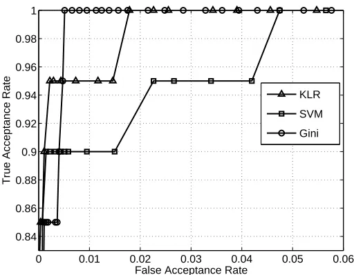
Figure 9: Comparison of ROC obtained for a speaker verification system based on soft-margin SVM and GiniSVM classification for speaker id: 148.

KLR, the average EER was computed to be equal to 0.36% and 0.35%, where as the EER for a

GiniSVM based system was found to 0.28%. This demonstrates that the normalization procedure used by GiniSVM improves the accuracy of a text-independent speaker verification system. The verification results are also comparable with other reported results on the YOHO data set (Campbell et al., 2002).

7. Conclusions and Extensions

We introduced a general, maximum entropy based framework for constructing multi-class support vector machines that generate normalized scores. In particular, GiniSVM produces direct estimates of conditional probabilities that approximate kernel logistic regression (KLR) at reduced com-putational cost, incurring quadratic programming under linear constraints as with standard SVM training. Unlike a baseline soft-margin SVM based system with calibrated probabilities, GiniSVM produces unbiased probability estimates owing to symmetry in the agnostic distance metric in the maximum entropy formulation. The probability estimates are sparse, where the number of non-zero probabilities is controlled by a single parameterγ, which acts as a margin in the normalization of probability scores. The margin parameter γis distinct from the regularization parameter C also

found in soft-margin SVM and KLR, even though both C andγweigh the agnostic metric relative

to the prior metric in the maximum entropy primal cost function.

re-duced precision implementation of SVMs. GiniSVM also successfully trained on a task of text-independent speaker verification, by integrating normalized probability scores over time. GiniSVM further extends to forward decoding kernel machines for trainable dynamic probabilistic inference on graphs (Chakrabartty and Cauwenberghs, 2002).

The maximum entropy framework for large-margin kernel probability regression introduced for GiniSVM is general and can be extended to other classification and regression tasks based on polynomial entropy. Of particular interest are formulations that use symmetric potential functions like the Gini quadratic entropy function.

Acknowledgments

This work was supported by grants from the Catalyst Foundation (http://www.catalyst-foundation.org), the National Science Foundation, and the Office of Naval Research.

Appendix A. Kernel Logistic Regression Primal and Dual Formulation

Proof of Proposition I: Define Le as the regularized log-likelihood/cross entropy for kernel logistic

regression (Wahba, 1998; Zhu and Hastie, 2002)

Le= M

∑

k=1

1 2||wk||

2_−C

∑

N

i=1

[ M

∑

k=1

yikfk(xi)−log(ef1(xi)+...+efM(xi))]. (30)

First order conditions with respect to parameters wkand bk in fk(x) =wk.x+bk yield

wk = C

N

∑

i=1

[yik−

efk(xi)

∑M p efp(xi)

]xi,

0 = C

N

∑

n [yik−

efk(xi)

∑M p efp(xi)

]. (31)

Denote

λn

k =C[yik−

efk(xi)

∑M p efp(xi)

] (32)

in the first-order conditions (31) to arrive at the kernel expansion (17) with linear constraint

fk(x) =

∑

n

λn

kK(xi,x) +bk, (33)

0 =

∑

n

λn k .

Note also that∑M_k=1λn_k=0 by construction.

Legendre transformation of the primal objective function (30) in wk and bk leads to a dual

formulation directly in terms of the coefficients λn

k (Jaakkola and Haussler, 1999). Define zn=

log(∑M_p efp(xi)_{), and Q}

i j=K(xi,xj). Then (32) and (33) transform to

∑

l

which correspond to first-order conditions of the convex dual functional

He= M

∑

k=1

[1 2 N

∑

n N

∑

l λn

kQnlλlk+C N

∑

n

(ynk−λnk/C)log(ynk−λnk/C)]

under constraints

∑

n

λn

k = 0, (34)

∑

k

λn

k = 0, (35)

λn

k ≤ Cynk

where bk and znserve as Lagrange parameters for the equality constraints (34) and (35).

Appendix B. GiniSV M Primal and Dual Formulation

Proof of Proposition II: The hinge function[.]+ can be appropriately modeled by introducing slack

variables µik≥0 into the loss function such that

Lg(wk,bk,zi) =min µik≥0

1 2

∑

_k |wk|

2₊γC

2

∑

_ik(yik− 1

γ[fk(xi)−zi+µik])2+

∑

ik

ηikµik

The first order conditions corresponding to the variables wk,bk,zi,µikare given by

∂F/∂wk = wk−C

N

∑

i=1

yik−

1

γ[fk(xi)−zi+µik]

xi=0, (36)

∂F/∂bk = C N

∑

i=1

yik−

1

γ[fk(xi)−zi+µik]

=0, (37)

∂F/∂zi = C

∑

k

yik−

1

γ[fk(xi)−zi+µik]

=0 (38)

∂F/∂µik = ηik−

1

γ[fk(xi)−zi+µik] =0 (39)

where ηik are the Lagrange multipliers corresponding to the inequality conditions µik ≥0. The

complementary slackness criterion (Bertsekas, 1995) for these constraints givesηik≥0 andηikµik=

0 which along with criterion (39) gives

1

γ[fk(xi)−zi+µik] =

1

γ[fk(xi)−zi]+≥0 (40)

and, according to (38),

∑

k

1

γ[fk(xi)−zi]+=1

which proves the first part of the proposition. To prove the second part of the proposition let

λi

k=Cyik−

1

Criteria (37), (38) and (40) lead to the constraints (11). Substitution in (36) yields an expansion of

wkwhich re-substituted in the primal yields the dual first-order condition

∑

j

Qi jλ_kj+bk−zi+µki −γ(yik−λik/C) =0.

Along with constraints (11) the corresponding dual reduces to the GiniSVM dual Hg (19), which

completes proof of the proposition.

Appendix C. Binary GiniSVM Dual Formulation

For a binary GiniSVM the dual cost function (19) becomes

Hg=

1 2C

∑

_{i j} λ

i +1λ

j +1Qi j+

1 2C

∑

_{i j} λ

i

−1λ

j

−1Qi j+

γ

2

∑

_i (yi,+1−λ

i

+1/C)2+

γ

2

∑

_i (yi,−1−λ

i

−1/C)2 (42) and the constraints (11) are written as

λi

−1=−λi+1, (43)

N

∑

i=1

λi

−1=

N

∑

i=1

λi

+1=0, (44)

λi

+1≤Cyi,+1, (45)

λi

−1≤Cyi,−1. (46)

Let λi =yiλi₊1 where yi = (2yi,+1−1). Then f(x) = 1₂(f+1(x)−f−1(x)) reduces to the kernel expansion (24) with b= 1₂(b+1−b−1). For binary labels yi=±1 the equality and inequality

con-straints (43)-(46) simplify to

N

∑

i=1

λi_y i=0,

0≤λi≤C.

Further substitution ofλi₊₁=yiλi, λi₋₁ =−yiλi, yi,+1= 1₂(1+yi) and yi,−1= 1₂(1−yi) into the binary GiniSVM dual cost function (42)

Hg=

1 C

∑

_{i j} λ

i_λj_y

iyjQi j−γ N

∑

i=1

1 2

2 −

1

2−

λi

C

2!

which is equivalent to the form Hb(25).

Appendix D. GiniSVM Sequential Minimum Optimization

The following extends the original SMO algorithm (Platt, 1999b) from binary soft-margin SVM to multi-class GiniSVM.

jointly updated. Without loss of generality the parameters of this working set will be referred to as

λ1∗

1 ,λ12∗,λ21∗ andλ22∗, where the indices correspond to k1,k2 and i1,i2. The aim of an SMO update is to find a new estimate of these coefficientsλ1₁,λ1

2,λ21 andλ22such that the new set of coefficients affect a net decrease in the objective function Hg(19), while still satisfying constraints C (11). This

is ensured by

λ1

1+λ12 = ζ1=λ11∗+λ12∗

λ1

1+λ21 = ξ1=λ11∗+λ21∗

λ1

2+λ22 = ξ2=λ12∗+λ22∗

λ2

2+λ21 = ζ2=λ22∗+λ21∗.

Only three of the above equalities need to be satisfied as the fourth one is automatically satisfied. Decomposing the GiniSVM dual in terms of these four coefficients leads to

H = 1

2Q11(λ 1

1)2+Q12λ11λ21+ 1 2Q22(λ

2

1)2+λ11

∑

j6=1,2

Q1 jλ₁j+λ2₁

∑

j6=1,2

Q2 jλ₁j

+ 1

2Q11(λ 1

2)2+Q12λ12λ22+ 1 2Q22(λ

2

2)2+λ12

∑

j6=1,2

Q1 jλ2j+λ 2 2

∑

j6=1,2 Q2 jλ2j

+ γC(y11−λ11/C)2+γC(y21−λ21/C)2+γC(y12−λ12/C)2+γC(y22−λ22/C)2. Substituting

λ1

2 = ζ1−λ11,

λ2

1 = ξ1−λ11,

λ2

2 = ξ2−ζ1+λ11 and using the first order condition∂H/∂λ1

1=0, optimal values forλ11∗are found as

λ1∗

1 =λ11+ (g12+g21−g11−g22)/2η (47) where

glm=−2γylm+

∑

j

Ql jλmj +2γ/Cλlm

and

η=Q11+Q22−2Q12+4γ/C.

At each step of the update (47) the GiniSVM dual function decreases, and repeated sampling of the four-point working set over the training set ensures proper convergence to the true minimum, barring degeneracies in the cost function. At convergence the parameters bk,k=1, ..,M are obtained

by solving a set of overcomplete equations for data points that lie in the interior of the boundary constraintsλi_k<Cyik. For the interior points denoted by its training index i the following condition

is satisfied

bk−zi+gik=0

which is over-complete in parameters bk,k=1, ..,M and zi,i=1, ..,I, where I denotes the total

References

E.L. Allwein, R.E. Schapire, and Y. Singer. Reducing multiclass to binary: A unifying approach for margin classifiers. Journal of Machine Learning Research, 1:113-141, 2000.

M. Alvira and R. Rifkin. An empirical comparison of SNoW and SVMs for face detection. CBCL paper 193 /AI Memo 2001-2004, MIT, 2001.

R. Auckenthaler, M. Carey and H. Lloyd-Thomas. Score normalization for text-independent speaker verification system. Digital Signal Processing, 10(1):42-54, 2000.

L.E. Baum and G. Sell. Growth transformations for functions on manifolds. Pacific J. Math., 27(2):211-227, 1968.

D. Bertsekas. Non-linear Programming. Athena Scientific, MA, 1995.

B. Boser, I. Guyon and V. Vapnik. A training algorithm for optimal margin classifier. Proc. 5th Ann. ACM Workshop on Computational Learning Theory (COLT), pages 144-52, 1992.

L. Breiman, J.H. Friedman and R. Olshen. Classification and Regression Trees. Wadsworth and Brooks, Pacific Grove CA, 1984.

C. Burges. A tutorial on support vector machines for pattern recognition. U. Fayyad, Ed., Proc. Data Mining and Knowledge Discovery, pages 1-43, 1998.

W.M. Campbell, K.T. Assaleh and C.C. Broun. Speaker with polynomial classifiers. IEEE Trans. Speech and Audio Proc., 10(4):205-212, May 2002.

G. Cauwenberghs and T. Poggio. Incremental and decremental support vector machine learning. Adv. Neural Information Processing Systems 10, Cambridge MA: MIT Press, 2001.

S. Chakrabartty and G. Cauwenberghs. Forward decoding kernel machines: A hybrid HMM/SVM approach to sequence recognition. IEEE Int. Conf. of Pattern Recognition: SVM workshop. (ICPR’2002), 2002.

S. Chakrabartty and G. Cauwenberghs. Margin propagation and forward decoding in analog VLSI. Proc. IEEE Int. Symp. Circuits and Systems (ISCAS’2004), 2004.

S. Chakrabartty and G. Cauwenberghs. Sub-microwatt analog VLSI support vector machine for pattern classification and sequence estimation. Adv in Neural Information Processing Systems 17, Cambridge: MIT Press, 2005.

T.M. Cover and J.A. Thomas, Elements of Information Theory. John Wiley and Sons, 1991.

K. Crammer and Y. Singer. The learnability and design of output codes for multiclass problems. Proc. 13th Ann. Conf. Computational Learning Theory (COLT), 2000.

T.G. Dietterich and G. Bakiri. Solving multiclass learning problems via error-correcting output codes. Journal of Artificial Intelligence Research, 2:263-286, 1995.

P.S. Gopalakrishnan, D. Kanevsky, A. Nadas and D. Nahamoo. An inequality for rational func-tions with applicafunc-tions to some statistical estimation problems. IEEE Trans. Information Theory, 37(1):107-113, 1991.

Y. Gu and T. Thomas. A text-independent speaker verification system using support vector machines classifier. Proc. Eur. Conf. Speech Communication and Technology (Eurospeech’01), pages 1765-1769, 2001.

C. Hsu and C. Lin. A comparison of methods for multi-class support vector machines. IEEE Trans. Neural Networks, 13(2):415-425, 2002.

P.J. Huber. Robust Estimation of Location Parameter. Annals of Mathematical Statistics, volume 35, 1964.

T. Jaakkola and D. Haussler. Probabilistic kernel regression models. Proc. 7th Int. Workshop on Artificial Intelligence and Statistics, 1999.

E. Jaynes. Information theory and statistical mechanics. Physics Review, 106:620-630, 1957.

T. Jebara. Discriminative, generative and imitative learning. PhD Thesis, MIT Media Laboratory, 2001.

T. Joachims. Text categorization with support vector machines. Technical Report LS-8 23, Univ. of Dortmund, 1997.

T. Joachims. Making large-scale support vector machine learning practical, In Sch ¨olkopf, Burges and Smola, Eds., Advances in Kernel Methods: Support Vector Machines, Cambridge MA: MIT Press, 1998.

M.I. Jordan and R.A. Jacobs. Hierarchical mixtures of experts and the EM algorithm. Proc. Int. Joint Conference on Neural Networks, 2:1339-1344, 1993.

S.S. Keerthi, S.K. Shevade, C. Bhattacharyya and K.R.K. Murthy. Improvements to Platt’s SMO algorithm for SVM classifier design. Neural Computation, 13:637-649, 2001.

J.T.Y. Kwok. Moderating the outputs of support vector machine classifiers. IEEE Transactions on Neural Networks, 10(5):1018-1031, 1999.

T. Nayak and C.R. Rao. Cross entropy, dissimilarity measures and characterizations of quadratic entropy. IEEE Trans. Information Theory, IT-31:589-593, 1985.

N. Lawrence, M. Seeger and R. Herbrich. Fast sparse gaussian process methods: The informative vector machine. Neural Information Processing Systems 15, pages 609-616, 2003.

M. Oren, C. Papageorgiou, P. Sinha, E. Osuna and T. Poggio. Pedestrian detection using wavelet templates. Computer Vision and Pattern Recognition (CVPR),pages 193-199, 1997.

E. Osuna, R. Freund and F. Girosi. Training support vector machines: An application to face detec-tion. Computer Vision and Pattern Recognition, pages 130-136, 1997.