A Scoring Function for Learning Bayesian Networks based on Mutual Information and Conditional Independence Tests

A Scoring Function for Learning Bayesian Networks based on Mutual

Information and Conditional Independence Tests

Luis M. de Campos [email protected]

Departamento de Ciencias de la Computación e Inteligencia Artificial E.T.S.I. Informática y de Telecomunicaciones, Universidad de Granada 18071-Granada, Spain

Editor: Nir Friedman

Abstract

We propose a new scoring function for learning Bayesian networks from data using score+search algorithms. This is based on the concept of mutual information and exploits some well-known properties of this measure in a novel way. Essentially, a statistical independence test based on the chi-square distribution, associated with the mutual information measure, together with a property of additive decomposition of this measure, are combined in order to measure the degree of inter-action between each variable and its parent variables in the network. The result is a non-Bayesian scoring function called MIT (mutual information tests) which belongs to the family of scores based on information theory. The MIT score also represents a penalization of the Kullback-Leibler di-vergence between the joint probability distributions associated with a candidate network and with the available data set. Detailed results of a complete experimental evaluation of the proposed scor-ing function and its comparison with the well-known K2, BDeu and BIC/MDL scores are also presented.

Keywords: Bayesian networks, scoring functions, learning, mutual information, conditional in-dependence tests

1. Introduction

Nowadays, Bayesian networks (Jensen, 1996; Pearl, 1988) constitute a widely accepted formalism for representing knowledge with uncertainty and efficient reasoning. A Bayesian network comprises a qualitative and a quantitative component. While the qualitative part represents structural informa-tion about a problem domain, in the form of causality, relevance or (in)dependence relainforma-tionships between variables, the quantitative part (which allows us to introduce uncertainty into the model) represents probability distributions that quantify these relationships. Once a complete Bayesian net-work has been built, it is an efficient tool for performing inferences. However, there still remains the previous problem of building such a network, that is, to provide the graph structure and the numerical parameters necessary for characterizing it. As it may be difficult and time-consuming to build Bayesian networks using the method of eliciting opinions from domain experts, and given the increasing availability of data in many domains, directly learning Bayesian networks from data is an interesting alternative.

associated with Bayesian networks, the search being guided by a scoring function that evaluates the degree of fitness between each element in this space and the available data.

The aim of this work is to define and study a new scoring function to be used by this class of Bayesian network learning algorithms as a competitive alternative to existing scoring functions (Bouckaert, 1993, 1995; Buntine, 1991; Chow and Liu, 1968; Cooper and Herskovits, 1992; Fried-man and Goldszmidt, 1996; HeckerFried-man et al., 1995; Herskovits and Cooper, 1990; Lam and Bac-chus, 1994; Suzuki, 1993). We also want to empirically evaluate the merits of the new score by means of a comparative experimental study.

The proposed scoring function is based on the concept of mutual information. This measure has several interesting properties, the most important for our purposes being the possibility of building a statistical test of independence based on the chi-square distribution. Mutual information has already been used either directly or indirectly within Bayesian network learning algorithms based on score and search (Bouckaert, 1993; Chow and Liu, 1968; Lam and Bacchus, 1994). The associated statis-tical test has also been used by several learning algorithms based on conditional independence tests (Acid and de Campos, 2001; Cheng et al., 2002; de Campos and Huete, 2000; Spirtes et al., 1993). However, what is new is the simultaneous quantification of the results of a set of independence tests based on mutual information. Basically, we use mutual information in order to measure the degree of interaction between each variable and its parent variables in the network, but penalizing this value using a term related to the chi-square distribution. This penalization term takes into account not only the network complexity but also its reliability. The result will undoubtedly be a scoring function, but any score+search-based algorithm using it will have some similarities with the learning methods based on independence tests (although we believe that our scoring function makes better use of the information provided by the tests than these methods). To a certain extent what we are proposing is a hybrid algorithm (either an algorithm based on scoring independences and search or an algorithm based on quantitative conditional independence tests).

Sections 2 and 3 of this paper provide some background about learning Bayesian networks and types of scoring functions, respectively. Section 4 covers the development of the new scoring func-tion, which we shall call MIT (mutual information tests). Section 5 carries out an empirical com-parative study of MIT against several state-of-the-art scoring functions (K2, BDeu and BIC/MDL). We first define the performance measures to be used and we then describe the corresponding exper-imental designs and the obtained results. Section 6 contains our conclusions and some proposals for future research. Finally, Appendix A includes proof of all the theorems set out in the paper.

2. Learning Bayesian Networks

Let us consider a finite set Un={X1,X2, . . . ,Xn}of discrete random variables.1 A generic variable of the set Unwill be denoted as either Xi or X . The domain of each variable Xi is a finite set Vi=

{xi1, . . . ,xiri}. A generic element of Viwill be denoted as xi. In general, we shall use uppercase letters

to denote variables, lowercase letters to denote states of the variables, and bold-faced letters (either uppercase or lowercase) to denote sets (of either variables or states of the variables, respectively).

A Bayesian network (BN) is a graphical representation of a joint probability distribution (Pearl, 1988) that includes two components:

• First, a directed acyclic graph (DAG) G= (Un,EG), where Un, the set of nodes, represents

the system variables,2 and EG, the set of arcs, represents direct dependency relationships between variables; the absence of arcs linking pairs of variables in turn represents the ex-istence of conditional independence relationships between these variables. A conditional independence relationship between two variables Xi and Xj, given a subset of variables Z, denoted as I(Xi,Xj|Z), means that given the values of the variables in Z, our degree of be-lief about the possible values of Xi is not modified once we know the value of variable Xj: p(xi|xj,z) = p(xi|z). Each variable Xi ∈Un has an associated parent set in the graph G,

PaG(Xi) ={Xj∈Un|Xj→Xi∈EG}. If Xihas no parent (it is a root node), then PaG(Xi) = /0.

• The second component is a set of numerical parameters, which usually represent conditional probability distributions: for each variable Xi in Un, we store a family of conditional

distri-butions p(Xi|paG(Xi)), one for each possible configuration,3 paG(Xi), of the parent set of Xi in the graph. If Xi has no parent, then p(Xi|paG(Xi))equals p(Xi). From these conditional distributions, we can obtain the joint distribution over Unusing:

p(x1,x2, . . . ,xn) =

∏

p(xi|paG(Xi))

The problem of learning Bayesian networks from data consists in finding the BN that (according to certain criterion) best fits the available data. This problem has been studied in depth over the last ten years and consequently, there are currently a considerable number of learning algorithms. As Bayesian networks have two different components (the graphical and the numerical model), the algorithms for learning BNs must deal with two different but highly related tasks: learning the structure (the DAG) and learning the parameters (the conditional probabilities). These two tasks cannot be carried out completely independently: on the one hand, in order to estimate the conditional probabilities, we must know the graphical structure; on the other, in order to determine whether the graph we are trying to find contains certain arcs, we need to estimate certain statistics from the data which, depending on the kind of learning algorithm being used, will be employed either to carry out some conditional independence tests or to measure the intensity of the relationships between the nodes involved in these arcs.

In this paper, we are only interested in algorithms for learning the structure of Bayesian net-works. As we mentioned previously, most of these algorithms can be grouped into two different categories: methods based on conditional independence tests (also called constraint-based meth-ods) and methods based on scoring functions and search, although there are also algorithms that use a combination of independence-based and scoring-based methods with different hybridization strategies (Acid and de Campos, 2000, 2001; Dash and Druzdzel, 1999; de Campos et al., 2003; Singh and Valtorta, 1995; Spirtes and Meek, 1995).

The algorithms based on independence tests (Cheng et al., 2002; de Campos, 1998; de Cam-pos and Huete, 2000; Meek, 1995; Pearl and Verma, 1991; Spirtes et al., 1993; Verma and Pearl, 1990; Wermuth and Lauritzen, 1983) perform a qualitative study of the dependence and indepen-dence relationships between the variables in the domain (obtained from the data by means of con-ditional independence tests), and attempt to find a network that represents these relationships as far as possible. Two fundamental issues for these algorithms are the number and the complexity of

2. In the same way, we shall represent a variable and its associated node in the graph.

the independence tests, and this can also cause unreliable results. Nevertheless, constraint-based algorithms generally come with rigorous theoretical founding and have developed a body of work that details sound and complete methods to make use of independence relations in the data while correctly accounting for structure.

The algorithms based on a scoring function attempt to find a graph that maximizes the selected score, which is usually defined as a measure of fitness between the graph and the data. All of them use the scoring function in combination with a search method in order to measure the goodness of each explored structure from the space of feasible solutions. Different learning algorithms are ob-tained depending on the search procedure used, as well as on the definitions of the scoring function and the search space.

The scoring functions are based on different principles, such as entropy and information (Chow and Liu, 1968; Herskovits and Cooper, 1990), the minimum description length (Bouckaert, 1993, 1995; Friedman and Goldszmidt, 1996; Lam and Bacchus, 1994; Suzuki, 1993), or Bayesian ap-proaches (Buntine, 1991; Cooper and Herskovits, 1992; Heckerman et al., 1995; Kayaalp and Cooper, 2002). The most usual scoring functions will be described later in more detail.

As far as the search is concerned, although the most frequently used are local search methods (Buntine, 1991; Chickering et al., 1995; Cooper and Herskovits, 1992; de Campos et al., 2003; Heckerman et al., 1995) due to the exponentially large size of the search space, there is a growing interest in other heuristic search methods such as simulated annealing (Chickering et al., 1995), tabu search (Acid and de Campos, 2003; Bouckaert, 1995), branch and bound (Tian, 2000), genetic algorithms and evolutionary programming (Larrañaga et al., 1996; Myers et al., 1999; Wong et al., 1999), Markov chain Monte Carlo (Kocka and Castelo, 2001; Myers et al., 1999), variable neighborhood search (de Campos and Puerta, 2001a), ant colony optimization (de Campos et al., 2002), greedy randomized adaptive search procedures (GRASP) (de Campos et al., 2002), and estimation of distribution algorithms (Blanco et al., 2003).

Most learning algorithms employ different search methods but the same search space: the DAG space. Possible alternatives are the space of the orderings of the variables (de Campos et al., 2002; de Campos and Huete, 2002; de Campos and Puerta, 2001b; Friedman and Koller, 2003; Larrañaga et al., 1996), with a secondary search in the DAG space compatible with a given ordering; the space of essential graphs (Pearl and Verma, 1990) (also called patterns or completed PDAGs), which are partially directed acyclic graphs4or PDAGs that canonically represent equivalence classes of DAGs (Andersson et al., 1997; Chickering, 2002; Dash and Druzdzel, 1999; Madigan et al., 1996; Spirtes and Meek, 1995); and the space of RPDAGs (restricted PDAGs), which also represent equivalence classes of DAGs (Acid and de Campos, 2003; Acid et al., 2005).

3. Scoring Functions for Learning Bayesian Networks

Focusing on the methods for learning Bayesian networks based on the score+search paradigm, the problem can be formally expressed as follows: given a complete5training data set D={u1, . . . ,uN}

of instances of Un, find a DAG G∗such that

G∗=arg max G∈Gn

g(G : D),

where g(G : D)is the scoring function measuring the degree of fitness of any candidate DAG G to the data set, and

G

The learning algorithms that search in the DAG space with local search-based methods can be more efficient if the scoring function being used has the property of decomposability: a scoring function g is decomposable if the value assigned to each structure can be expressed as a sum (in the logarithmic space) of local values that depend only on each node and its parents:

g(G : D) =

∑

Xi∈Un

g(Xi,PaG(Xi): D)

g(Xi,PaG(Xi): D) =g(Xi,PaG(Xi): N_XD_i,PaG(Xi)),

where ND

Xi,PaG(Xi)are the sufficient statistics of the set of variables{Xi} ∪PaG(Xi)in D, that is, the

number of instances in D corresponding to each possible configuration of{Xi} ∪PaG(Xi).

For example, a search procedure that only changes one arc at each move can efficiently evaluate the improvement obtained by this change. It can reuse most of the previous computations and only the statistics for the variables whose parent sets have been modified must be recomputed. In this way, the insertion or deletion of an arc Xj →Xi in a DAG G can be evaluated by computing only one new local score, g(Xi,PaG(Xi)∪ {Xj}: D)or g(Xi,PaG(Xi)\ {Xj}: D), respectively; the reversal of an arc Xj→Xirequires the evaluation of two new local scores, g(Xi,PaG(Xi)\ {Xj}: D) and g(Xj,PaG(Xj)∪ {Xi}: D).

Another property which is particularly interesting if the learning algorithm searches in a space of equivalence classes of DAGs is called the score equivalence: a scoring function g is score-equivalent if it assigns the same value to all DAGs that are represented by the same essential graph. In this way, the result of evaluating an equivalence class will be the same regardless of which DAG from this class is selected.

There are different ways to measure the degree of fitness of a DAG with respect to a data set. Most can be grouped into two categories: Bayesian and information measures. We shall use the following notation: the number of states of the variable Xiis ri; the number of possible configura-tions of the parent set PaG(Xi)of Xiis qi; obviously, qi=∏Xj∈PaG(Xi)rj; wi j, j=1, . . .qi, represents

a configuration of PaG(Xi); Ni jk is the number of instances in the data set D where the variable Xi takes the value xik and the set of variables PaG(Xi) take the value wi j; Ni j is the number of in-stances in the data set where the variables in PaG(Xi) take their j-th configuration wi j; obviously Ni j=∑rki=1Ni jk; similarly, Nikis the number of instances in D where the variable Xi takes its k-th value xik, and therefore Nik=∑q_j=i ₁Ni jk; the total number of instances in D is N.

3.1 Bayesian Scoring Functions

Starting from a prior probability distribution on the possible networks, the general idea is to compute the posterior probability distribution conditioned to the available data D, p(G|D). The best network is the one that maximizes the posterior probability. It is not in fact necessary to compute p(G|D) and for comparative purposes, computing p(G,D)is sufficient since the term p(D)is the same for all the possible networks. As it is easier to work in the logarithmic space, in practice, the scoring functions use the value log(p(G,D))instead of p(G,D).

network structure), and can be expressed as follows:

gK2(G : D) =log(p(G)) + n

∑

i=1

"_q i

∑

j=1

"

log

(ri−1)! (Ni j+ri−1)!

+ ri

∑

k=1

log Ni jk!

##

, (1)

where p(G)represents the prior probability of the DAG G. Afterwards, the so-called BD (Bayesian Dirichlet) score was proposed by Heckerman et al. (1995) as a generalization of K2:

gBD(G : D) =log(p(G)) + n

∑

i=1

" _q i

∑

j=1

"

log

Γ(η

i j) Γ(Ni j+ηi j)

+ ri

∑

k=1 log

Γ(N

i jk+ηi jk) Γ(ηi jk)

##

, (2)

where the valuesηi jkare the hyperparameters for the Dirichlet prior distributions of the parameters given the network structure, andηi j=∑rki=1ηi jk.Γ(.)is the function Gamma,Γ(c) =

R∞

0 e−uuc−1du. It should be noted that if c is an integer,Γ(c) = (c−1)!. If the values of all the hyperparameters are ηi jk=1, we obtain the K2 score as a particular case of BD.

In practical terms, the specification of the hyperparameters ηi jk is quite difficult (except if we use non-informative assignments, as the ones employed by K2). However, by considering the ad-ditional assumption of likelihood equivalence (Heckerman et al., 1995), it is possible to specify the hyperparameters relatively easily. While the result is a scoring function called BDe (and its expres-sion is identical to the BD one in Equation 2), the hyperparameters can now be computed in the following way:

ηi jk=η×p(xik,wi j|G0),

where p(.|G0)represents a probability distribution associated with a prior Bayesian network G0and ηis a parameter representing the equivalent sample size.

A particular case of BDe which is especially interesting appears when p(xik,wi j|G0) =_ri1_qi, that is, the prior network assigns a uniform probability to each configuration of{Xi} ∪PaG(Xi). The resulting score is called BDeu, which was originally proposed by Buntine (1991). This score only depends on one parameter, the equivalent sample sizeη, and is expressed as follows:

gBDeu(G : D) =log(p(G)) + n

∑

i=1

"_q i

∑

j=1

"

log Γ(

η

qi)

Γ(Ni j+_qη_i)

!

+ ri

∑

k=1

log Γ(Ni jk+

η

riqi)

Γ(_rη

iqi)

!##

. (3)

Regarding the term log(p(G))which appears in all the previous expressions, it is quite common to assume a uniform distribution (except if we really have information about the greater desirability of certain structures) so that it becomes a constant and can be removed.

3.2 Scoring Functions based on Information Theory

of the model and the description length of the data given the model. Complex models usually require greater description lengths but reduce the description length of the data given the model (they are more accurate). On the other hand, simple models require shorter description lengths but the description length of the data given the model increases. The minimum description length principle establishes an appropriate trade-off between complexity and precision.

In our case, the data set to be represented is D and the selected class of models are Bayesian networks. Therefore, the description length includes the length required to represent the network plus the length necessary to represent the data given the network (Bouckaert, 1993, 1995; Friedman and Goldszmidt, 1996; Lam and Bacchus, 1994; Suzuki, 1993). In order to represent the network, we must store its probability values, and this requires a length which is proportional to the number of free parameters of the factorized joint probability distribution.6 This number, called network complexity and denoted as C(G), is:

C(G) = n

∑

i=1

(ri−1)qi.

The usual proportionality factor is 1₂log(N)(Rissanen, 1986). Therefore, the description length of the network is:

1

2C(G)log(N).

Regarding the description of the data given the model, by using Huffmann codes its length turns out to be the negative of the log-likelihood, that is, the logarithm of the likelihood function of the data with respect to the network. This value is minimum for a fixed network structure when the network parameters are estimated from the data set itself by using maximum likelihood. The log-likelihood can be expressed in the following way (Bouckaert, 1995):

LLD(G) = n

∑

i=1 qi

∑

j=1 ri

∑

k=1 Ni jklog

Ni jk Ni j

. (4)

Therefore, the MDL scoring function (by changing the signs to deal with a maximization problem) is:

gMDL(G : D) = n

∑

i=1 qi

∑

j=1 ri

∑

k=1 Ni jklog

Ni jk Ni j

−1

2C(G)log(N). (5)

Another way of measuring the quality of a Bayesian network is to use measures based on in-formation theory and some of these are closely related with the previous one. The basic idea is to select the network structure that best fits the data, penalized by the number of parameters which are necessary to specify the joint distribution. This leads to a generalization of the scoring function in Equation 5:

g(G : D) = n

∑

i=1 qi

∑

j=1 ri

∑

k=1 Ni jklog

Ni jk Ni j

−C(G)f(N), (6)

where f(N)is a non-negative penalization function. If f(N) =1, the score is based on the Akaike information criterion (AIC) (Akaike, 1974). If f(N) = 1

2log(N), then the score, called BIC, is

based on the Schwarz information criterion (Schwarz, 1978), which coincides with the MDL score. If f(N) =0, we have the maximum likelihood score, although this is not very useful as the best network using this criterion is always a complete network which includes all the possible arcs.

It is interesting to note that another way of expressing the log-likelihood in Equation 4 is:

LLD(G) =−N n

∑

i=1

HD(Xi|PaG(Xi)), (7)

where HD(Xi|PaG(Xi)) represents the conditional entropy of the variable Xi given its parent set PaG(Xi), for the probability distribution pD:

HD(Xi|PaG(Xi)) = qi

∑

j=1

pD(wi j) − ri

∑

k=1

pD(xik|wi j)log(pD(xik|wi j))

!

,

and pD is the joint probability distribution associated with the data set D, obtained from the data by maximum likelihood. The log-likelihood LLD(G)can also be expressed as follows (Bouckaert, 1995):

LLD(G) =−NHD(G),

where HD(G)represents the entropy of the joint probability distribution associated with the graph G when the network parameters are estimated from D by maximum likelihood:

HD(G) =−

∑

n

∏

i=1

pD(xi|paG(Xi))

!

log n

∏

i=1

pD(xi|paG(Xi))

!!

.

Therefore, another interpretation of the scoring functions based on information is that they attempt to minimize the conditional entropy of each variable given its parents, and so they search for the par-ent set of each variable that gives as much information as possible about this variable (or which most restricts the distribution). It is necessary to add a penalization term since the minimum conditional entropy is always obtained after adding all the possible variables to the parent set.

An alternative way to avoid this overfitting without using a penalization function was proposed by Herskovits and Cooper (1990) who used the maximum likelihood score, but the process of insert-ing arcs into the network was stopped by means of a statistical test, which determined whether the difference in entropy between the current network and the one obtained by including an additional arc was statistically significant.

With respect to the characteristics of the different scoring functions, all are decomposable and with the exception of K2 and BD, they are also score-equivalent (Chickering, 1995).

4. A New Scoring Function based on Mutual Information and Independence Tests

In order to explain the ideas behind the proposed scoring function more clearly, we shall first intro-duce several preliminary considerations. These will lead to a first version of the scoring function, which will be later refined in order to obtain the final version.

4.1 Preliminary Considerations

joint probability distribution associated with the data, pD. We should mention that pG must be understood to be the joint probability distribution that factorizes according to G and whose local conditional probability distributions are estimated from D by means of maximum likelihood, that is,

pG(x1, . . . ,xn) = n

∏

i=1

pD(xi|paG(Xi)).

A reasonable choice for the distance measure is the Kullback-Leibler divergence (Kullback, 1968):

KL(pD,pG) =

∑

x1,...,xn

pD(x1, . . . ,xn)log

pD(x1, . . . ,xn) pG(x1, . . . ,xn)

.

This distance can also be expressed in another more convenient way:

KL(pD,pG) = −HD({X1, . . . ,Xn}) + n

∑

PaG(_Xi)=/0

HD(Xi)

+ n

∑

PaG(_Xi)6=/0

HD({Xi} ∪PaG(Xi))−HD(PaG(Xi))

, (8)

where HD(X)represents the entropy of the set of variables X with respect to the distribution pD. We shall now consider the concept of mutual information. Given a probability distribution p defined over two sets of variables X and Y, the mutual information between X and Y is:

MI(X,Y) =

∑

x,y

p(x,y)log

p(x,y)

p(x)p(y)

,

which can also be expressed in terms of entropy as:

MI(X,Y) =H(X) +H(Y)−H(X∪Y). (9)

Mutual information (which is simply the Kullback-Leibler divergence between the joint distribution for X and Y and the product of the corresponding marginals) can be considered as a way of mea-suring the dependence degree between the sets of variables X and Y, which is null when the two sets of variables are independent and maximum when they are functionally dependent. By using Equation 9, we can rewrite Equation 8 as follows (Lam and Bacchus, 1994):

KL(pD,pG) =−HD({X1, . . . ,Xn}) + n

∑

i=1

HD(Xi)− n

∑

PaG(_Xi)6=/0

MID(Xi,PaG(Xi)). (10)

As the two first terms in Equation 10 do not depend on the DAG G being considered, we obtain:

arg min G∈Gn

KL(pD,pG) =arg max G∈Gn

n

∑

PaG(Xi)6=/0

MID(Xi,PaG(Xi)), (11)

We have still not achieved anything useful, however, since mutual information has the property that MI(X,Y∪W)≥MI(X,Y), in other words, mutual information always increases by including additional variables. Therefore, the complete network will always have minimum Kullback-Leibler divergence with respect to the data. In fact, by taking into account Equation 7 and the relation between mutual information and conditional entropy, namely MI(X,Y) =H(X)−H(X|Y), we can write:

n

∑

PaG(Xi)6=/0

MID(Xi,PaG(Xi)) =

LLD(G)

N +

n

∑

i=1

HD(Xi). (12)

Therefore, minimizing the Kullback-Leibler divergence is also equivalent to maximizing log-likelihood. The following expression is equivalent to the previous one:

n

∑

PaG(_Xi)6=/0

MID(Xi,PaG(Xi)) = 1 N

n

∑

i=1 qi

∑

j=1 ri

∑

k=1 Ni jklog

N Ni jk NikNi j

.

However, there are certain advantages to using mutual information instead of log-likelihood as we shall see later. First, let us consider the concept of conditional mutual information between X and Y given a set of variables Z, defined as:

MI(X,Y|Z) =

∑

z

p(z)

∑

x,y

p(x,y|z)log

p(x,y|z) p(x|z)p(y|z)

!

,

which can be expressed by MI(X,Y|Z) =H(X|Z)−H(X|Y∪Z), and also by:

MI(X,Y|Z) =H(X∪Z) +H(Y∪Z)−H(Z)−H(X∪Y∪Z).

The following property7of conditional mutual information is important for our purposes:

MI(X,Y∪W|Z) =MI(X,Y|Z) +MI(X,W|Z∪Y). (13)

Another fundamental property of mutual information is:

Theorem 1 (Kullback, 1968) Given a data set D with N elements, if the hypothesis that X and Y

are conditionally independent given Z is true, then the statistics 2N MID(X,Y|Z)approximates to a

distributionχ2(l)(Chi-square) with l= (rX−1)(rY−1)rZdegrees of freedom, where rX, rYand rZ

represent the number of configurations for the sets of variables X, Y and Z, respectively. If Z= /0,

the statistics 2N MID(X,Y)approximates to a distributionχ2(l)with l= (rX−1)(rY−1)degrees

of freedom.

4.2 Developing a New Scoring Function

The basic idea underlying the new scoring function that we shall propose is very simple: to use the mutual information MID(Xi,PaG(Xi)) in order to measure the degree of interaction between each variable Xiand its parents PaG(Xi), as in Equation 11, but penalizing this value using a term related

7. It should be noted that this property is a numeric version of the properties of decomposition, weak union and

con-traction of the probabilistic independence relationships and other dependence models (Pearl, 1988). These three

to the χ2 distribution. This term attempts to re-scale the mutual information values in order to prevent these values from systematically increasing as the number of variables in PaG(Xi)does.

In our opinion, one problem with the scoring functions based on information (Equation 6) is that they penalize log-likelihood globally, with a combination of the network complexity and a function that depends only on the number of instances. Since we believe that as the log-likelihood can be decomposed as a sum of components (each being associated with a variable and its parents), then each of these components should be penalized differently, depending not only on its complexity but also on its reliability. For example, a DAG where a variable Xihas many parents is always penalized in the same way, without taking into account to what extent this topology is actually necessary to adequately and reliably represent the distribution for Xi. The scoring function that we shall propose naturally incorporates this kind of penalization, and is based on solid statistical grounds.

Given a DAG G, let us consider the mutual information between a variable Xi and its parents, MID(Xi,PaG(Xi)). Let sibe the number of parent variables8of Xi, si=|PaG(Xi)|. Let us assume that PaG(Xi) ={Xi1, . . . ,Xisi}. By iteratively applying Equation 13, we can express MID(Xi,PaG(Xi))as:

MID(Xi,PaG(Xi)) = MID(Xi,{Xi1, . . . ,Xisi})

= MID(Xi,{Xi1, . . . ,Xi(si−1)}) +MID(Xi,Xisi|{Xi1, . . . ,Xi(si−1)})

= MID(Xi,{Xi1, . . . ,Xi(si−2)}) +MID(Xi,Xi(si−1)|{Xi1, . . . ,Xi(si−2)}) +

MID(Xi,Xisi|{Xi1, . . . ,Xi(si−1)}) =. . . .

= MID(Xi,Xi1) + si

∑

j=2

MID(Xi,Xi j|{Xi1, . . . ,Xi(j−1)}). (14)

The elements in this decomposition of the mutual information will be interpreted as follows: start-ing with an empty set of parents of Xi, we have first included the arc Xi1→Xi, and the degree of dependence between these variables is MID(Xi,Xi1). We then insert the arc Xi2→Xi and as Xi1 is already a parent of Xi, the dependence degree between Xi2 and Xi is MID(Xi,Xi2|Xi1). We continue inserting arcs in this way until the last one Xisi →Xi(with a dependence degree between Xisi and Xi

equal to MID(Xi,Xisi|{Xi1, . . . ,Xi(si−1)})) has been included. If we do not insert any additional arcs,

this is because each remaining variable Xhdoes not contribute any additional information9with re-spect to Xi, this information being measured as MID(Xi,Xh|{Xi1, . . . ,Xisi}). The key question is how

to determine whether the values of mutual information represent an appreciable (i.e., statistically significant) amount of information. At this point, we can use the result in Theorem 1.

We know that 2NMID(Xi,Xi j|{Xi1, . . . ,Xi(j−1)})approximates to a distributionχ2(li j), with the appropriate degrees of freedom li j. Let us fix a confidence levelαand determine the valueχα,li j such

that p(χ2_(l

i j)≤χα,li j) =α. This does in fact represent a statistical test of conditional independence:

if 2NMID(Xi,Xi j|{Xi1, . . . ,Xi(j−1)})≤χα,li j, then we accept the hypothesis of independence between

Xiand Xi j given{Xi1, . . . ,Xi(j−1)}(with probabilityα); otherwise we reject it.

The use of this kind of independence test within BN learning algorithms is quite frequent (Acid and de Campos, 2001; de Campos and Huete, 2000; Spirtes et al., 1993). It has also been used by algorithms based on score+search to stop the search process (Acid and de Campos, 2000; Herskovits and Cooper, 1990). The problem with an independence test is that it only asserts whether the

8. sishould not be confused with qi, which represents the number of configurations of these variables.

variables are independent or not, rather than quantifying the extent to which they are. For example, if an algorithm is trying to decide which of the two variables Xjand Xk to exclude from the parent set of another variable Xi, if both variables turn out to be dependent on Xi(given its current parent set), the test is not able to discriminate between them, although it may be possible for one variable to be more closely dependent on Xithan the other.

Our proposal is to quantify the result of the independence test to build the scoring function. The difference 2NMID(Xi,Xi j|{Xi1, . . . ,Xi(j−1)})−χα,li j gives us a measure of the degree of interest for

adding the variable Xi j to the current parent set of Xi: if the difference is negative (the test would say that Xi and Xi j are independent), the score will decrease, and the more clearly independent the variables are, the more it will decrease; when the difference is positive (the test would assert that these two variables are dependent), the score will increase, and the more dependent Xiand Xi j are, the more it will increase.

Therefore, a measure of the global quality of the set PaG(Xi)as the parent set of variable Xiis:

g(Xi,PaG(Xi): D) = si

∑

j=2

2N MID(Xi,Xi j|{Xi1, . . . ,Xi(j−1)})−χα,li j

+2N MID(Xi,Xi1)−χα,li1, (15)

whereχ_α,li j is the value such that p(χ

2_(l

i j)≤χα,li j) =α, and the number of degrees of freedom is:

li j=

(ri−1)(ri j−1)∏_kj−₌1₁rik j=2, . . . ,si (ri−1)(ri1−1) j=1 .

(16)

The expression in Equation 15 is then a global quantification of a series of si simultaneous condi-tional independence tests, and by virtue of the decomposition of mutual information in Equation 14, it is equivalent to:

g(Xi,PaG(Xi): D) =2N MID(Xi,PaG(Xi))− si

∑

j=1

χα,li j. (17)

The scoring function would therefore be defined according to Equation 11 as:

g(G : D) = n

∑

PaG(Xi)6=/0

2N MID(Xi,PaG(Xi))− si

∑

j=1 χα,li j

. (18)

It should be noted that although the value of mutual information will increase after new variables are added to the parent set, the penalization component (which contains one term for each parent variable) will also increase. In this way, we are able to appropriately re-scale the mutual information measure.

The value of α, which represents the confidence level associated with the statistical test, is a free parameter that may be fixed to any standard value (for example 0.90, 0.95 or 0.99). However, since we are in fact performing several simultaneous tests (as many as the number of variables in PaG(Xi)), and also taking into account the Bonferroni inequality,10in order for the global confidence level to be acceptable (that is to say, a reasonably high value of p(∩si

j=1(χ2(li j)≤χα,li j))), it will be

necessary forαto be greater than the standard values used when performing a single test.

10. p(∩n

i=1Ai)≥1−∑ni=1

1−p(Ai)

In order to accurately compute the values χα,l, we can use a standard method which is based on the algorithm proposed by Hill and Pike (1965, 1985) to compute the chi-squared integral (i.e., the probability p(χ2_{(l)>x)) in combination with a simple bisection search. Alternatively, if speed} is more important than great accuracy, as the χ2(l) distribution can be approximated by several transformations of the standardized normal distribution N(0,1)for large degrees of freedom (Evans et al., 1993), we can use tabulated exact values for l≤100 and the Wilson-Hilferty approximation (which is quite accurate) for l>100:

χ2_(l)≈lh₁₋ 2 9l+

r

2

9lN(0,1)

i3

.

4.3 The MIT Score

Throughout the previous discussion, we have omitted one very important detail: the decomposi-tion of mutual informadecomposi-tion that we have used (Equadecomposi-tion 14) is not unique and we can decompose MID(Xi,PaG(Xi))in many other ways - as many as the number of possible orderings of the variables in PaG(Xi), that is, si!. Each corresponds to a different way of including the variables in the parent set of Xi one at a time. The ordering does not affect the value MID(Xi,PaG(Xi)), but it can affect the penalization component (this will be the case whenever the number of states rikof all the variables is not the same). By way of example, let us assume that PaG(Xi) ={X1,X2,X3}. The six possible decompositions of MID(Xi,{X1,X2,X3})are:

MID(Xi,X1) +MID(Xi,X2|X1) +MID(Xi,X3|{X1,X2})

MID(Xi,X1) +MID(Xi,X3|X1) +MID(Xi,X2|{X1,X3}) MID(Xi,X2) +MID(Xi,X1|X2) +MID(Xi,X3|{X1,X2}) MID(Xi,X2) +MID(Xi,X3|X2) +MID(Xi,X1|{X2,X3}) MID(Xi,X3) +MID(Xi,X1|X3) +MID(Xi,X2|{X1,X3}) MID(Xi,X3) +MID(Xi,X2|X3) +MID(Xi,X1|{X2,X3}).

Let us suppose that the number of states of the variables Xi, X1, X2 and X3 is ri=3, r1=2, r2=3 and r3=4. The penalization component in Equation 17 for each of the six previous decompositions is therefore:

χα,2+χα,8+χα,36=107.93 χα,2+χα,12+χα,32=109.21 χα,4+χα,6+χα,36=108.91 χα,4+χα,18+χα,24=111.96 χα,6+χα,8+χα,32=111.07 χα,6+χα,16+χα,24=112.89.

The numerical values in these expressions are computed for the parameter α=0.999. It should be noted that the total number∑si

j=1li j of degrees of freedom is always the same, 46 in this case, which would correspond to the degrees of freedom of a marginal independence test between Xi and PaG(Xi); such a test would use(ri−1)(∏sj=i 1ri j−1)degrees of freedom11(the value ofχα,46

11. Observe that∑si

j=1li j=∑sji=1

(ri−1)(ri j−1)∏kj−=11rik

in the example is 81.40). In any case, the values are different since the chi-square distribution is not additive with respect to the number of degrees of freedom.12 Therefore, depending on the selected ordering, the score in Equation 17 will be different. This is undesirable since the same DAG (depending on the path that the search process follows to reach it) would be evaluated differently. In order to solve this problem, we believe that the best we can do is to use the most conservative option, that is, to use the greatest of all these values so as to evaluate each parent set in the worst possible way.

In order to formalize this idea, letσi= (σi(1), . . . ,σi(si))denote any permutation of the index set(1, . . . ,si)of the variables in PaG(Xi) ={Xi1, . . . ,Xisi}, and let us define:

l_iσi(j)=

(ri−1)(riσi(j)−1)∏

j−1

k=1riσi(k) j=2. . . ,si

(ri−1)(riσi(1)−1) j=1 .

(19)

Then, instead of using Equation 17, the global quality measure of the set PaG(Xi)that we propose is:

g(Xi,PaG(Xi): D) =2N MID(Xi,PaG(Xi))−max_σ

i

si

∑

j=1

χα,liσ_i(j).

The final expression of the proposed scoring function, which we shall call MIT (from mutual infor-mation tests), is:

gMIT(G : D) = n

∑

PaG(_Xi)6=/0

2N MID(Xi,PaG(Xi))−max

σi

si

∑

j=1 χα,liσi(j)

. (20)

Computing each penalization component maxσi∑

si

j=1χα,liσi(j) in the previous expression might seem

to be a very time-consuming task since it would be necessary to evaluate all the si! possible permu-tations of the variables in the set PaG(Xi)in order to calculate the maximum. Fortunately, this will not be necessary as this maximum can be obtained in a much simpler way:

Theorem 2 For the values liσi(j)defined in Equation 19,

max

σi

si

∑

j=1

χα,liσ_i(j)=

si

∑

j=1 χα,l_iσ∗

i(j),

where σ∗_i is any permutation of PaG(Xi) satisfying riσ∗i(1)≥riσ∗i(2)≥. . .≥riσ∗i(si), whenever the

function fi,α:

N

R

si

j=1χα,lj, is a Shur-concave function.

This result says that the permutation that produces the maximum penalization value is the one where the first variable has the greatest number of states, the second variable has the second largest number of states, and so on. In the previously considered example, this permutation is{X3,X2,X1}, and this reaches a maximum value equal to 112.89.

The combination of theoretical and empirical arguments that support this conjecture is included in the Appendix. The restriction concerningαdoes not represent any practical problem since we shall always use values ofαwhich are much greater than 0.59.

Another way of measuring the quality of a set of variables Z as the parent set of Xi, which as it turns out is equivalent to the previous one, is as follows: we can consider that Z will be a good parent set if it continues to be a good parent set when one of its variables is removed, Z\ {Y}, and also the variable Y that we have removed should not have been removed, that is, Y is not independent of Xi given Z\ {Y}. As we can do this for each variable in Z, the final value should be the smallest one (we are again using a conservative or pessimistic view). This leads to a recursive definition of g(Xi,PaG(Xi): D). The way of measuring the degree of undesirability of removing the variable

Y from Z is to use the difference between the mutual information statistic 2N MID(Xi,Y|Z\ {Y})

and the chi-square valueχ_α,l with the appropriate degrees of freedom. In this way, if Y is truly independent on Xi given Z\ {Y}, then this difference will be negative and in this case we would prefer to use Z\ {Y} instead of Z as the parent set of Xi. If, on the contrary, the difference is positive, the set Z will be preferable to Z\ {Y}.

We can therefore recursively define the score gr(Xi,PaG(Xi): D)in the following way:

gr(Xi,PaG(Xi): D) = min Xi j∈PaG(Xi)

n

gr(Xi,PaG(Xi)\ {Xi j}: D) +

2N MID(Xi,Xi j|PaG(Xi)\ {Xi j})−χα,li jr o

, (21)

whereχα,lr

i j is the value such that p(χ

2_(lr

i j)≤χα,lr

i j) =αand the number of degrees of freedom is

lr_{i j}= (ri−1)(ri j−1)∏ski=1

k6=j

rik. The starting point of this recursive definition is obviously gr(Xi,/0:

D) =0. We can prove the following result:

Theorem 4 The MIT scoring function defined in Equation 20 can also be expressed as: gMIT(G : D) =

n

∑

PaG(Xi)6=/0

gr(Xi,PaG(Xi): D),

where gr(Xi,PaG(Xi): D)are the local scores defined in Equation 21.

Let us study some of the properties of the MIT score.

Theorem 5 The MIT scoring function defined in Equation 20 is decomposable.

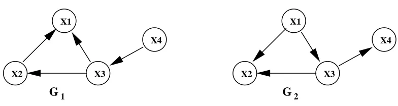
Unfortunately, MIT is not score-equivalent. Let us consider the following example: for the two DAGs G1and G2in Figure 1 and which are equivalent, let us suppose that the number of states of each variable is: r1=5, r2=4, r3=3, r4=2. Therefore:

g(G1: D) = 2N(MID(X1,{X2,X3}) +MID(X2,X3) +MID(X3,X4))

−(χ_α,12+χα,32+χα,6+χα,2)

g(G2: D) = 2N(MID(X2,{X1,X3}) +MID(X3,X1) +MID(X4,X3))

−(χ_α,12+χα,30+χα,8+χα,2).

X4 X1

X2 X3

X4 X1

X2 X3

G

G_{1 2}

Figure 1: Two equivalent DAGs with different values of the MIT score

likelihood score is score-equivalent. The problem appears with the penalization by means of the sum of chi-square values: if the variables have a different number of states (as in this case), the results are different. More specifically, the penalization component is 131.67 for G1but 132.55 for G2(assuming thatα=0.999).

The MIT score, however, satisfies a less demanding property than score-equivalence, and this concerns another type of space of equivalent DAGs, namely RPDAGs (Acid and de Campos, 2003). They are PDAGs which represent sets of equivalent DAGs, although they are not a canonical rep-resentation of equivalence classes of DAGs (two different RPDAGs may correspond to the same equivalence class). Let us introduce some additional notation and then the concept of RPDAG. The skeleton of a DAG is the undirected graph that results from ignoring the directionality of every arc. A h-h pattern (head-to-head pattern) in a DAG G is an ordered triplet of nodes,(Xi,Xk,Xj), such that G contains the arcs Xi→Xk and Xj→Xk. Given a PDAG G= (Un,EG), for each node Xi∈Un,

SibG(Xi) ={Xj ∈Un|Xi—Xj ∈EG} is the set of siblings or neighbors of Xi. A PDAG G is an RPDAG if and only if it satisfies the following conditions:

1. ∀Xi∈Un, if PaG(Xi)6=/0then SibG(Xi) =/0.

2. G contains neither directed nor completely undirected cycles.

3. ∀Xi,Xj∈Un, if Xj∈PaG(Xi)then either|PaG(Xi)| ≥2 or PaG(Xj)6=/0.

The difference between essential graphs and RPDAGs appears when there are triangular structures: essential graphs may have completely undirected cycles, but these cycles must be chordal (Anders-son et al., 1997). In other words, undirected cycles are forbidden in RPDAGs, whereas in essential graphs only undirected non-chordal cycles are forbidden. It can be seen that all the DAGs which are represented by a given RPDAG are equivalent and have the same skeleton and the same h-h patterns, wh-hereas th-he DAGs associated with-h an essential graph-h h-have th-he same skeleton and th-he same v-structures (h-h patterns where the extreme nodes are not adjacent) (Pearl and Verma, 1990). Therefore, the role played by the v-structures in essential graphs is the same as that played by the h-h patterns in RPDAGs. The objective of RPDAGs is to trade the uniqueness of the representation of equivalence classes of DAGs for a more manageable one, because testing whether a given PDAG G is an RPDAG is easier than testing whether G is an essential graph.

Theorem 6 The MIT scoring function assigns the same value to all DAGs that are represented by the same RPDAG.

To conclude our study of the new score, we have observed an interesting relation between MIT and the scoring functions based on Equation 6. First, it should be noted that the log-likelihood of the simplest possible network, namely the empty network G_/0, is, according to Equation 4 (and taking into account that in this case qi=1 and Ni jk=Nik):

LLD(G/0) = n

∑

i=1 ri

∑

k=1 Niklog

Nik N

=−N n

∑

i=1

HD(Xi).

Then, considering Equation 12, we can express the sum of mutual information measures between each variable and its set of parents in G as follows:

n

∑

PaG(Xi)6=/0

MID(Xi,PaG(Xi)) =

LLD(G)−LL(G/0)

N .

Therefore, the sum of mutual information measures coincides with the difference between the log-likelihood of G and the one of G/0or, equivalently, with the difference between the description length of the data given G/0and given G. Now, let us consider the difference between G and G/0in terms of complexity, which is:

C(G)−C(G/0) =

n

∑

i=1

(ri−1)qi− n

∑

i=1

(ri−1) = n

∑

PaG(Xi)6=/0

(ri−1)(qi−1) = n

∑

PaG(Xi)6=/0

si

∑

j=1 li j,

with li jdefined as in Equation 16. Therefore, for the information-based scoring function defined in Equation 6, using f(N) =1/2, the difference between the scores of G and G/0is:

g(G : D)−g(G/0: D) =LL(G)−C(G)f(N)−LL(G/0)−C(G/0)f(N)

=N n

∑

PaG(_Xi)6=/0

MID(Xi,PaG(Xi))− 1 2

n

∑

PaG(_Xi)6=/0

si

∑

j=1 li j

=1 2

n

∑

PaG(_Xi)6=/0

2N MID(Xi,PaG(Xi))− si

∑

j=1 li j

. (22)

The similarity of this expression with those in Equations 18 and 20 is apparent. Therefore, the MIT score of a network G could be interpreted in terms of the difference between the information-based scores of G and G_/0, and also as the decrease in description length achieved by using G instead of G/0. By considering that the mean value of aχ2distribution with l degrees of freedom is just l, we can see that the MIT score appears when we replace in Equation 22 the mean values of theχ2(li j) distributions by the correspondingα-quantiles.

5. Experimental Evaluation

prior distribution over possible structures and as this score is quite sensitive with respect to the value of the equivalent sample size, we shall use five values of this parameter, more preciselyη= 1,2,4,8,16. For the single parameter of the MIT score (i.e., the confidence level), we shall use three values:α=0.99,0.999,0.9999.

The software necessary to carry out the experiments has been developed on the Elvira system (Elvira, 2002), a Java tool for building and using Bayesian networks and influence diagrams.

First, we define the performance criteria that we shall use to compare the different scoring functions.

5.1 Performance Criteria

One way of measuring the quality of a scoring function is to study its ability to reconstruct (in com-bination with a learning algorithm based on score+search) the Bayesian network which generated the data. In other words, we begin with a Bayesian network G0 which is completely specified in terms of structure and parameters, and we obtain a data set of a given size by sampling from G0. Then, using the scoring function together with a search method, we obtain a learned network G, which must be compared with the original network G0. This capacity for reconstruction can be understood in two different but complementary ways: reconstructing the graphical structure and reconstructing the associated joint probability distribution. In terms of the first of these, the usual evaluation consists in measuring the structural differences between the original and the learned net-works. More precisely, the number of added arcs (A(G)), deleted arcs (D(G)), and inverted arcs (I(G)) in the learned network with respect to the original one is computed. In order to eliminate fictitious differences or similarities between the two networks regarding the number of inverted arcs (caused by different but equivalent subDAG structures), before the two networks are compared they will be converted into their corresponding essential graph representation using the algorithm pro-posed by Chickering (1995). If G0 and G0₀represent the essential graphs associated with G and G0, respectively, then the three measures of structural difference can be calculated using the following expressions:

A(G) =1

2 n

∑

i=1

|AdG0(X_i)\Ad_G0

0(Xi)|

D(G) =1

2 n

∑

i=1

|Ad_G0

0(Xi)\AdG0(Xi)|

I(G) = n

∑

i=1

|Pa_G0

0(Xi)∩SibG0(Xi)|+|PaG0(Xi)∩SibG00(Xi)|+|PaG00(Xi)∩ChG0(Xi)|

.

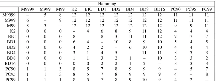
where ChH(Xi) ={Xj∈Un|Xi→Xj∈EH}and AdH(Xi) =PaH(Xi)∪ChH(Xi)∪SibH(Xi)are the sets of children and adjacent nodes of Xi in a PDAG H. As a way of summarizing these three measures, the Hamming distance, which is simply the sum of all the structural differences, H(G) =

A(G) +D(G) +I(G), is also usually considered.

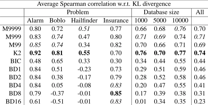
In terms of the ability to reconstruct the joint probability distribution, we can evaluate this by means of a distance measure between the distributions associated with the original and the learned networks, pG0 and pG, respectively. We shall use the Kullback-Leibler divergence:

KL(G) =KL(pG0,pG) =

∑

x1,...,xn

pG0(x1, . . . ,xn)log

pG0(x1, . . . ,xn) pG(x1, . . . ,xn)

The conditional probability distributions that constitute the factorization of pG will be calculated from the data set using the Laplace estimation (Good, 1965), which avoids the problem of obtaining an infinite value of the Kullback-Leibler divergence, caused by zero probability values in pG.

The calculus of this distance measure for joint distributions with many variables is computa-tionally very expensive. However, by taking advantage of the factorization of the distributions, the complexity may be considerably reduced and the value KL(G)can be expressed as follows:

KL(G) = n

∑

i=1 ri

∑

k=1 qG0i

∑

j=1

pG0(xik,wG0i j )log(pG0(xik|wG0i j ))

−

n

∑

i=1 ri

∑

k=1 qG

i

∑

j=1

pG0(xik,wGi j)log(pG(xik|wGi j)),

where wG0_{i j} and wG_{i j}represent the j-th configuration of the parent sets of Xiin G0and G, respectively (each having a total number of possible configurations equal to qG0_i and qG_i , respectively). In this way, the only probability values that must be computed are pG0(xik,wG0i j )and pG0(xik,wGi j), and this can be done relatively efficiently by using a propagation algorithm in the network G0. We have used an exact algorithm based on variable elimination.

One alternative way of measuring the quality of a scoring function which does not require an initial Bayesian network to be used as a starting point is to use the network learned with such a scoring function for a specific task and then to evaluate the level of success achieved. As Bayesian networks have been used in different ways to build classifiers, we can evaluate the quality of a scor-ing function (at least in comparative terms) by buildscor-ing a classifier usscor-ing an algorithm for learnscor-ing Bayesian networks which is specific for classification and equipped with the scoring function, and then measuring its classification capacity.

5.2 Experiments for Reconstructing Bayesian Networks

In order to make our comparative study more representative, we shall use different problems or rather different original networks. We shall also use different database sizes. Although this parame-ter clearly affects the quality of the networks learned with any scoring function (greaparame-ter sizes lead to better estimations), we want to check which of the scoring functions may be more or less sensitive in the sense that their behavior deteriorates more quickly when smaller sample sizes are used.

In the following sections, we shall first give details of the experimental design before presenting the obtained results.

5.2.1 EXPERIMENTALDESIGN

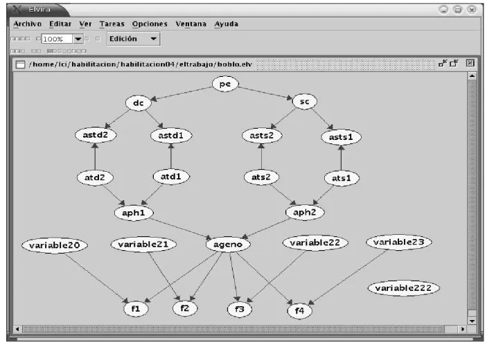
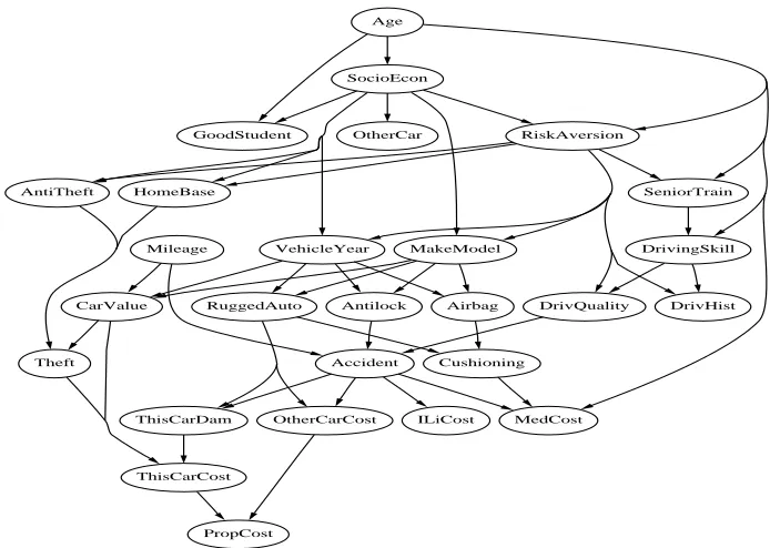
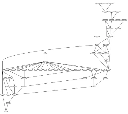
We have selected four Bayesian networks corresponding to different problems: Alarm (Figure 2), Boblo (Figure 3), Insurance (Figure 4) and Hailfinder (Figure 5).

1 2 3

25 18 26

17

19 20

10 21

27

28 29

7 8 9

30

32

12

34 35

33 14

22

15

23 13

16

36

24

6 5 4 11

31

37

Figure 2: The Alarm network

is a network for evaluating car insurance risks. The Insurance network contains 27 variables and 52 arcs. All these networks have been widely used in specialist literature for comparative purposes.

Figure 3: The Boblo network

SocioEcon

GoodStudent RiskAversion

VehicleYear MakeModel AntiTheft HomeBase

OtherCar Age

DrivingSkill SeniorTrain

MedCost

DrivQuality DrivHist RuggedAuto Antilock

CarValue Airbag

Accident

ThisCarDam OtherCarCost ILiCost

ThisCarCost

Cushioning Mileage

PropCost Theft

Figure 4: The Insurance network

The search method that we shall use is a local search in the DAG space with the classical operators of arc addition, arc deletion and arc reversal. The starting point of the search is always the empty graph. Although our main objective is to compare the proposed score with others, given that MIT has some similarities with constraint-based methods, it is also interesting to include one of these methods in the comparison. We have selected the well-known PC algorithm (Spirtes et al., 1993). This algorithm also depends on one parameter αrepresenting the confidence level of the independence tests. We shall use three values:α=0.90,0.95,0.99.

We therefore have a design 13×4×3 (10 scoring functions plus 3 versions of a constraint-based algorithm, 4 problems and 3 sample sizes), and for each of these 156 configurations we use 5 different databases, which gives us a total of 780 experiments.

5.2.2 RECONSTRUCTIONRESULTS

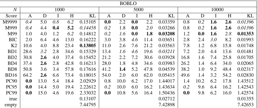
Tables 1, 2, 3 and 4 display the results obtained for the Alarm, Boblo, Hailfinder and Insurance networks, respectively. For each sample size and each method, each table shows the average values of the previously mentioned performance measures (A, D, I, H and KL). The best value for each performance measure is written in bold and the second best in italics. In the last two rows of each table, we also show the KL values for the original network (with parameters re-trained from the cor-responding database) and the empty network, which may serve as a kind of scale. Table 5 displays an illustrative summary of the results: it shows the number of times (from the 12 configurations being considered for each method) that each method has obtained the best result (and either the best or the second best result) for each of the five performance measures.

Scenario

MvmtFeatures MidLLapse ScenRelAMCIN Dewpoints

ScnRelPlFcst SfcWndShfDis RHRatio

ScenRelAMIns WindFieldPln TempDis SynForcng MeanRH LowLLapse

ScenRel3_4

WindFieldMt WindAloft

AMInsWliScen

InsSclInScen

PlainsFcst

InsChange AMCINInScen

CapInScen

CapChange CompPlFcst

AreaMoDryAir

CldShadeOth

InsInMt AreaMeso_ALS

CombClouds

MorningCIN

CldShadeConv OutflowFrMt

MountainFcst

WndHodograph

Boundaries CombMoisture

CurPropConv

N34StarFcst

LoLevMoistAd

MorningBound AMInstabMt

CombVerMo

LatestCIN LLIW

SatContMoist RaoContMoist

Date

R5Fcst

LIfr12ZDENSd AMDewptCalPl

VISCloudCov IRCloudCover N0_7muVerMo SubjVertMo

QGVertMotion

Figure 5: The Hailfinder network

since MIT with the values α=0.999,0.9999 offers better results than with α=0.99. It is also possible to observe how MIT generally behaves better than the other scores, with respect to all the performance measures, and more specifically, in terms of BIC/MDL (which is the closest scoring function in spirit to the new score), MIT systematically obtains much better results. Although BIC behaves acceptably in terms of the number of added arcs, it does however have a marked propensity to remove a large number of arcs. This suggests that the penalization component used by BIC is not well calibrated. On the other hand, the different versions of BDeu behave rather poorly (except in terms of the number of deleted arcs). K2 only offers good results for the KL divergence. The PC algorithm behaves very good for the number of added and inverted arcs. However, its results in terms of the number of deleted arcs and KL divergence are extremely poor.