Penalized Model-Based Clustering with Application to Variable Selection

Penalized Model-Based Clustering with Application to Variable

Selection

Wei Pan [email protected]

Division of Biostatistics School of Public Health University of Minnesota Minneapolis, MN 55455, USA

Xiaotong Shen [email protected]

School of Statistics University of Minnesota Minneapolis, MN 55455, USA

Editor: Bin Yu

Abstract

Variable selection in clustering analysis is both challenging and important. In the context of model-based clustering analysis with a common diagonal covariance matrix, which is especially suitable for “high dimension, low sample size” settings, we propose a penalized likelihood approach with an L1penalty function, automatically realizing variable selection via thresholding and delivering a

sparse solution. We derive an EM algorithm to fit our proposed model, and propose a modified BIC as a model selection criterion to choose the number of components and the penalization parameter. A simulation study and an application to gene function prediction with gene expression profiles demonstrate the utility of our method.

Keywords: BIC, EM, mixture model, penalized likelihood, soft-thresholding, shrinkage

1. Introduction

This article concerns variable selection in model-based clustering, especially for “high dimension, low sample size” data, where the data dimension greatly exceeds the number of observations. Specifically, given n P-dimensional observations xj= (xj1, ...,xjP)0for j=1, ...,n, we aim to group

the data into a few, say K, clusters such that the observations in the same cluster are more similar to each other than those from different clusters. In this context, some of the attributes xj p’s of xj may

and/or backward eliminations of variables, in model-based clustering; an alternative is to conduct best subset selection, which however is unrealistic for high-dimensional data: for example, with P=1000, there are more than 10300 possible models to be considered, which is prohibitive given the current standard computing power. Furthermore, even for smaller problems, as in regression, due to its discreteness, best subset selection may be unstable and may not work well in selecting relevant variables (Tibshirani, 1996); most importantly, unlike in regression or classification but unique to clustering or semi-supervised learning, best subset selection may identify a correct model which however is of no interest, as to be confirmed by our numerical example later.

With high-dimensional data, as an alternative to variable selection, one may apply dimension reduction techniques, such as principal component analysis, prior to clustering (Ghosh and Chin-naiyan, 2002; Liu et al., 2003). A possible drawback of this approach is the separation between dimension reduction and subsequent clustering; for example, as pointed out by many researchers (Chang, 1983; Yeung and Ruzzo, 2001; Raftery, 2003), using first few principal components in clustering may destroy the clustering structure of the original data.

There has been increasing interest in variable selection for model-based clustering, mostly within the Bayesian framework (Liu et al., 2003; Hoff, 2005, 2006; Tadesse et al., 2005; Raftery and Dean, 2006; Kim et al., 2006). An idea is to parametrize the mean of cluster k as µk=µ+δk,

where µ is the global mean. It is clear that, if some components ofδkare 0, then the corresponding

attributes are not informative to clustering, at least in terms of the means/locations. Two Bayesian approaches have been proposed based on this idea (Liu et al., 2003; Hoff, 2005, 2006). Another Bayesian approach, analogous to stepwise variable selection in regression, is to sequentially com-pare two nested models to determine whether an attribute should be included in or excluded from the current model based on a greedy search (Raftery and Dean, 2006), which may be computation-ally too time-consuming for high-dimensional data. In contrast, to our knowledge, no frequentist alternatives to subset selection are available for variable selection in model-based clustering. In light of the success of penalized regression with variable selection (Tibshirani, 1996; Fan and Li, 2001), we conjecture that penalization may be also viable to variable selection in clustering, and hence we propose an approach through penalized model-based clustering. Specifically, cluster-specific means µk are adaptively shrunken towards the global mean µ; with an appropriately chosen penalty

func-tion, some components of µkare estimated to be exactly the same as that of µ, effectively realizing

variable selection. We also propose a modified BIC as a model selection criterion to adaptively determine the amount of penalization as well as the number of clusters. Note that, although there is an extensive body of literature on penalized likelihood methods, most focus on classification and regression; in particular, to our knowledge, we are not aware of any existing works on penalized likelihood particularly designed for multivariate clustering.

facilitates interpretation of results, and even directly addresses biological questions of interest, for example, which genes are involved in the biology of a cancer or its subtypes. In this article, in addi-tion to the promising applicaaddi-tion of cancer subtype discovery, we also apply model-based clustering to the task of gene function discovery (Li and Hong, 2001; Ghosh and Chinnaiyan, 2002). Although the human genome and many other genome sequencing projects have led to a discovery of many new genes, biological functions of many genes remain unknown; many known functions also need to be refined. It has become popular to cluster gene expression profiles to discover unknown gene functions.

In the remaining parts of this article, we first review briefly the standard model-based clustering, then we introduce a general framework for penalized model-based clustering. We propose a spe-cific implementation with an L1penalty, resulting in soft-thresholding on the mean parameters, and thus realizing automatic variable selection. We derive an EM algorithm to compute the maximum penalized likelihood estimates for the model; a modified BIC is used to determine the number of components and the value of the penalization parameter in penalized model-based clustering. We compare the proposed method with the standard method using simulated data and gene expression data for tumor subtype discovery and gene function prediction; in particular, we illustrate problems associated with clustering without variable selection, and those with best subset selection, conclud-ing that penalized clusterconclud-ing is an effective and simple method for variable selection. We end the article with a short discussion on some open questions.

2. Methods

We first give a brief review on model-based clustering with a finite Normal mixture model, then we introduce our penalized model-based clustering, including an EM algorithm and a modified BIC for model selection.

2.1 Model-based Clustering

In model-based clustering, it is assumed that each observation x is drawn from a finite mixture dis-tribution f(x;Θ) =∑K

k=1πkfk(x;θk), with the mixing proportionπk, component-specific distribution

fk and its parametersθk. Denote byΘ={(πk,θk): k=1, ...,K}all unknown parameters, with

re-striction that 0≤πk ≤1 for any k and ∑Kk=1πk =1. Each component of the mixture distribution

corresponds to a cluster. The number of clusters, K, has to be determined in practice; see section 2.4.

Given data xj, j=1, ...,n, the log-likelihood is

log L(Θ) =

n

∑

j=1 log[

K

∑

k=1

πkfk(xj;θk)].

Maximization of the above log-likelihood with respect to Θis difficult, and it is common to use the EM algorithm (Dempster et al., 1977) by casting the problem in the framework of missing data. Define zk jas the indicator of whether xj is from component k; that is, zk j=1 if xj is indeed

from component k, and zk j=0 otherwise. If the missing data zk j’s could be observed, then the

log-likelihood for the complete data is:

log Lc(Θ) =

∑

∑

The EM algorithm can be applied to obtain the maximum likelihood estimator (MLE) ofΘ; see McLachlan and Peel (2002) and Fraley and Raftery (2002) for more details.

2.2 Penalized Model-based Clustering

With the same motivation as in penalized regression, we propose a penalized model-based cluster-ing approach. The general purpose of penalization is for model regularization, which in general can enhance the predictive power of a model, and may be even necessary in some situations. For exam-ple, in the univariate Normal mixture model with each fk(.) =φ(.; µk,σk), it is well-known that with

σk→0, we have a degeneracy with log L being unbounded, and thus no (unrestricted) MLE exists.

Ciuperca et al. (2003) proposed a penalized likelihood approach to dealing with the degeneracy: by penalizing small variance componentsσk, one circumvents the problem. In addition, as to be

discussed in the next section, with an appropriate choice of penalty function, we can realize a sparse solution, resulting in automatic variable selection.

Specifically, we regularize log L(Θ)to yield a penalized log-likelihood:

log LP(Θ) = n

∑

j=1 log[

K

∑

k=1

πkfk(xj;θk)]−hλ(Θ),

where h_λ()is a penalty function with penalization parameterλ. The choice of h_λ()depends on the goal of the analysis; see Fan and Li (2001) for some general theory. Correspondingly, the penalized log-likelihood for the complete data is

log Lc,P(Θ) = K

∑

k=1

n

∑

j=1

zk j[logπk+log fk(xj;θk)]−hλ(Θ).

We propose using such penalized model-based clustering as a general way to regularize parameter estimates. This can be useful for high-dimensional data, especially for situations of “large P, small n”. Recently Fraley and Raftery (2005) proposed a Bayesian approach to regularizing model-based clustering; there is a large body of literature on Bayesian mixture modeling, for example, Richard-son and Green (1997), Jasra et al. (2005) and references therein. There is a well known connection between penalized likelihood and Bayesian modeling (Hastie et al., 2001): it can be regarded that minus the penalty function −h_λ(Θ)is proportional to the log density of the prior distribution for parametersΘ, and the penalized (log) likelihood is proportional to the (log) posterior density.

Note that in contrast to Ciuperca et al. (2003), where only univariate Normal mixture models were considered, our main interest here is in multivariate clustering.

2.3 Penalizing Mean Parameters

Now we propose a specific implementation of penalized model-based clustering to realize variable selection. Consider the common case with each component fk as Normal. We are particularly

interested in “large P, small n” often encountered in genomic studies. Hence, as in naive Bayes classification, we adopt a working independence model for components of xj. Furthermore, to

sample mean 0 and sample variance 1. Specifically, we have

fk(x;θk) =

1

(2π)P/2_|V|exp

−1

2(x−µk)

0_V−1_(x−µ

k)

,

where V =diag(σ1,σ2, ...,σP), and|V|=∏Pp=1σp. We propose using the L1penalty: h_λ(Θ) =λ

∑

k

∑

though other penalty functions may be also suitable, as discussed in Fan and Li (2001) in the context of regression. The main goal is to obtain a sparse solution with many small estimates of µk p’s

automatically set to 0, thus realizing variable selection.

Next we derive an EM algorithm for the above penalized model-based clustering; in particular, it is confirmed that the L1-penalty yields a thresholding rule with the desired sparsity property. The derivation closely follows from that for standard model-based clustering (McLachlan and Peel, 2002) and the general methodology for penalized likelihood (Green, 1990). We use generic notation

Θ(m) _{to represent the parameter estimates at iteration m, and use X = (x}

1, ...,xn) to denote all the

observations. It is easy to verify that the E-step yields

QP(Θ;Θ(m)) =E_Θ(m)(log Lc,P|X) =

∑

∑

τ(m)

k j [logπk+log fk(xj;θk)]−λ

∑

∑

|µk p|,

where

τ(m)

k j =

π(m)

k fk(xj;θ

(m)

k )

f(xj;Θ(m))

= π (m)

k fk(xj;θ

(m)

k )

∑K k=1π

(m)

k fk(xj;θ

(m)

k )

(1)

is the estimated posterior probability of xj’s coming from component k.

The M-step maximizes the above QPto update the parameter estimates. It is easy to show that

∂QP

∂πk

=

∑

j

(τ(_{k j}m)/πk−τ(K jm)/πK),

for any k=1,2, ...,K−1, and

∂QP

∂σ2

p

=

∑

k

∑

τ(m)

k j "

− 1 2σ2

p

+(xj p−µk p) 2 2σ4

p #

,

for any p=1, ...,P. Hence

ˆ

π(m+1)

k =

n

∑

j=1

τ(m)

k j /n, and σˆ

2,(m+1)

p = K

∑

∑

τ(m)

k j (xj p−µ

(m)

k p )

2_{/n. (2)}

Now for the mean parameters,

∂QP

∂µk

=

∑

j

τ(m)

k j V

−1_(x

Some algebraic manipulations yield

ˆµ(_km+1)=sign(˜µ(_km+1))



|˜µ

(m+1)

k | −

λ ∑jτ

(m+1)

k j

V(m+1)1





+

, (3)

where ˜µ_k(m+1)=∑_jτ_{k j}(m+1)xj/∑jτ

(m+1)

k j is the usual update for µk if no penalty is imposed; for any

f , f+ = f if f >0, and f+ =0 otherwise; 1 is a vector with all elements 1’s. Note that all the operations in (3), including sign() and ()+, are component-wise. It is evident that, if λ>

|∑n j=1τ

(m+1)

k j xj p/σ

2,(m+1)

p |, then ˆµ(_{k p}m+1)=0; otherwise, ˆµ_{k p}(m+1) is obtained by shrinking ˜µ(_{k p}m+1)

to-wards 0 by an amountλσ2,(p m+1)/∑nj=1τ (m+1)

k j .

The above iteration is repeated until convergence, resulting in the maximum penalized likeli-hood estimate (MPLE) ˆΘ. Then we use (1) to calculate the posterior probability of any observation x’s belonging to each cluster, and assign the observation to the cluster with the highest probability. Because of possible existence of multiple local maxima, we run the algorithm multiple times, and each time we use the result from a randomly started K-means algorithm as starting values for the EM. We fit a series of models with various values of K andλ, then use a model selection criterion to choose their appropriate values, as to be discussed in the next section.

It can be seen that, if ˆµk p=0 for all k, then the p-th attribute does not contribute to clustering:

it will be cancelled out from the numerator and the denominator of (1). In contrast, in the standard method, all attributes contribute to the posterior probability calculation.

Note that in (3), if we use ˜µ(_km+1), instead of ˆµ(_km+1), we obtain the standard model-based cluster-ing, which is equivalent to usingλ=0. In our numerical examples, to reduce bias, we used ˜µ(_{k p}m)in (2) to estimateσ2_p, though we did not find much difference in several simulations if ˆµ(_{k p}m)was indeed used. In addition, if we replace ˆµ(_km+1)by

ˆµ(_km_,H+1)=˜µ(_km+1)I(λ>| n

∑

j=1

τ(m+1)

k j V

−1,(m)_x

j|),

we obtain so-called hard-thresholding, which is in contrast to soft-thresholding in (3). In our nu-merical examples, we found that hard-thresholding gave results similar to those of soft-thresholding, and we will skip its further discussion.

2.4 Model Selection

In practice, we need to determine the number of components, K. This is realized by first fitting a series of models with various numbers of components, and then using a model selection criterion to choose the best one. For standard model-based clustering, it is common to use Bayesian information criterion (BIC) (Schwarz, 1978) defined as

BIC=−2 log L(Θ˜) +log(n)d,

For penalized model-based clustering, in addition to K, we also have to choose an appropriate value of penalization parameterλ; a model selection criterion has to account for the adaptive choice ofλ. One difficulty in using the above BIC criterion is that it is not always clear what is d in a pe-nalized model. Although other resampling-based model selection methods, such as cross-validation or generalized degrees of freedom (Shen and Ye, 2002) can be employed, they are computationally more demanding, and even prohibitive for large and/or high-dimensional data as considered here. Following a conjecture of Efron et al. (2004) and a result of Zou et al. (2004) for L1-penalized re-gression, we treat d as the number of non-zero parameter estimates, modifying BIC for penalized model-based clustering as

BIC=−2 log L(Θˆ) +log(n)de,

where ˆΘ is the MPLE, and de=K+P+KP−1−q is the effective number of parameters; we

set q as the number of the MPLE mean components that equal to 0. Hence, as expected, due to thresholding, de<d with a large penalization parameterλ.

3. Results

We first present results for simulated data, then consider clustering samples and clustering genes for two microarray data.

3.1 Simulated Data

We consider first high-dimensional data, then, to facilitate comparisons with best subset selection, we also consider low-dimensional data.

3.1.1 LARGEP

We first considered simulated data as described in Hoff (2004) and Hoff (2005). In each simulated data set, there were two clusters based on the first 150 attributes, while only one cluster based on the remaining 850 attributes; in other words, there were a total of P=1000 variables with the first 150 effective while the other 850 as noise variables in forming two clusters. Specifically, there were n=100 observations with 85 in one cluster and 15 in the other: the first 150 variables were iid from N(0,1)for the first cluster, whereas they were iid from N(1.5,1) for the second cluster; the remaining 850 variables were all iid from N(0,1) for either cluster. Hence, there were 150 informative attributes and 850 noise ones.

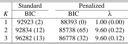
For each of 100 simulated data sets, we fitted a series of models with the number of components K=1, 2, 3 and various values of penalization parameterλ=0, 1, 1.5, 2, 5, 7.5, 10, 12.5, 15, 17.5, 20, 25 and 30.

Standard Penalized

K BIC BIC λ

1 92923 (2) 88393 (0) 1.00 (0.00) 2 92834 (12) 85738 (65) 9.60 (0.22) 3 96282 (13) 86778 (32) 9.60 (0.12)

Table 1: Mean BIC (with standard errors in parentheses) with various numbers (K) of clusters in the standard and penalized clustering for 100 simulated data sets. λis the value of the penalization parameter minimizing BIC for the given K.

Standard Penalized

K Freq BIC Freq BIC λ #Zero1 #Zero0

1 20 92923 0 - - -

-(5)

2 80 92791 94 85679 9.57 1.1 832.5

(10) (64) (0.22) (0.2) (1.7)

3 0 - 6 86348 7.50 0.0 626.5

(43) (0.00) (0.0) (5.6)

Standard Penalized

K Freq Freq #(1 and 2) #(1 or 2, not both) #Zero1 #Zero0

1 100 6 0 0 2 8

(0) (0)

2 0 38 30 6 0.26 5.08

(0.09) (0.26)

3 0 56 42 12 0.29 2.45

(0.07) (0.19)

Table 3: Frequencies of the selected numbers (K) of clusters in the standard and penalized clus-tering from 100 simulated data sets with P=10. The frequencies of the corresponding models including both the two informative attributes (#(1 and 2)), or only one of the two (#(1 or 2, not both)), and the means (with standard errors in parentheses) of the number of the two informative attributes excluded (#Zero1), and the number of the other 8 noise attributes excluded (#Zero0) are also included.

K=2, uncovering the interesting structure in the data. Importantly, the penalized approach can automatically select attributes: out of the total 850 noise attributes, on average, 833 attributes were correctly identified and not used in the final clustering; on the other hand, only one out of 150 informative attributes was not used.

Penalized clustering gave perfect assignments for K =2: the 15 and 85 observations from two distributions/classes were correctly assigned to clusters 1 and 2 respectively. More interestingly, even when K=3 was selected, the assignments were also correct; the clustering results for the 6 simulated data sets with K =3 were the following: i) for two data sets, the 15 observations from class 1 were assigned to cluster 1, and 45 and 40 observations from class 2 were assigned to clusters 2 and 3 respectively, denoted as{(15,0,0),(0,45,40)}; ii) for two data sets:{(15,0,0),(0,49,36)}; iii) for the other two,{(15,0,0),(0,48,37)}and{(15,0,0),(0,46,39)}respectively.

It would be interesting to compare our method with best subset selection, which however was computationally prohibitive: with 1000 attributes, there were 21000≈10300possible subsets/models! Note that, because there is no formal significance test for each individual attribute in model-based clustering, the commonly used sequential variable selection in regression is not applicable here. Below, we considered a problem with a much smaller P so that a comparison with best subset selection was possible.

3.1.2 SMALLP

Any attributes ≥2 attributes

K Freq #(1 and 2) #(1 or 2, not both) Freq #(1 and 2) #(1 or 2, not both)

1 79 0 0 56 11 6

2 19 0 7 41 21 11

3 2 0 1 3 2 0

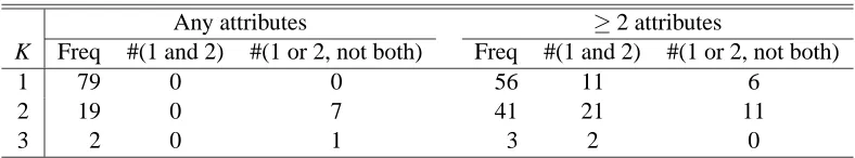
Table 4: Frequencies of the selected numbers (K) of clusters by best subset selection from 100 simulated data sets with P=10. The frequencies of the corresponding models including both the two informative attributes (#(1 and 2)), or only one of the two (#(1 or 2, not both)). Two searches were conducted: all possible models including any combinations of the attributes, and only models including at least two attributes.

Table 3 gives the results for standard and penalized clustering. Again, in presence of the eight noise attributes, standard clustering always chose K =1; in contrast, penalized clustering with automatic variable selection tended to chose K>1, and the two informative attributes were most often retained. However, penalized clustering did not work as well as in the previous set-up with P=1000: it chose K=3 most often while keeping most of the noise attributes; the reason could be that with fewer informative attributes, this was a more difficult problem than that of the previous section. Nevertheless, compared with best subset selection (Table 4), it still worked much better. In best subset selection, if we considered all possible non-null models (i.e., all possible non-null combinations of attributes), it most often selected K=1; in all cases, only one noise attribute was included in the selected model. Because there was indeed only one cluster according to any noise attribute, the choice of K=1 based on any noise attribute was correct; in other words, the selected model was correct, though of no interest. This highlights a unique point that in variable selection for clustering, unlike in regression, a correct model for the data based on a subset of attributes (e.g., noise attributes here) may be of no interest!

In addition, we considered only the models containing at least two attributes in best subset selection (Table 4). It turned out that all the selected models included only two attributes; it was still more likely to choose K=1, most often with two noise attributes, which was again caused by the the complication of having so many correct models of no interest: there was indeed only one cluster based on any two of the noise attributes. In summary, we concluded that subset selection was not suitable at all for variable selection in clustering, whereas penalized clustering was much more effective.

3.2 Tumor Subtype Discovery Using Gene Expression Profiles

Standard Penalized

K BIC BIC λ

1 76966 69691 >0

2 73802 68504 5

3 71104 66630 3

4 72232 65378 3

5 - 64034 2

6 - 62912 2

7 - 61950 2

8 - 63626 3

Table 5: BIC values for various numbers (K) of clusters in standard and penalized clustering for Golub’ gene expression data.

Standard Penalized

Samples/clusters 1 2 3 1 2 3 4 5 6 7

ALL 4 0 23 0 1 1 1 7 8 9

AML 0 4 7 6 0 0 0 4 1 0

Table 6: Clustering results for Golub’s data.

were not even expressed in any sample, we filtered out most genes: we ranked the genes based on their sample variances across all 38 samples, and used only the top 2000 ones. For each method, we started from g=1 and increased g until a minimum BIC was reached. The standard clustering chose K=3 while the penalized one selected K=7 (Table 5).

The clustering results are detailed in Table 6. The penalized method performed better than the standard clustering: the former incorrectly assigned five while the latter misclassified seven AML samples into the clusters with the ALL samples as the majority. In penalized clustering, although 35% of the mean parameter estimates were 0’s, only eight genes had their cluster-specific mean estimates as 0’s across all seven clusters, and hence were regarded as non-informative; previous studies demonstrated that there were indeed a large number of the genes differentially expressed between ALL and AML samples (Thomas et al., 2001; Pan, 2002).

3.3 Gene Function Discovery Using Gene Expression Profiles

learning problem, as opposed to supervised learning: first, we do not restrict the genes of the same function to be in the same cluster/class; each of the multiple clusters of the genes coming from the same functional category may suggest some novel subcategory, a refinement of the original func-tional category. Second, we allow the existence of some unknown and novel classes: some genes of unknown function do not have to be predicted to have any one of the known functions because they may have some unknown new functions. Here, we considered gene function discovery using gene expression data for yeast S cerevisiae. Specifically, we used a gene expression data set con-taining 300 microarray experiments with gene deletions and drug treatments (Hughes et al., 2000). Variable selection was highly relevant here: first, as shown in simulation, incorrectly using noise attributes might degrade the performance of clustering, obscuring some interesting clustering struc-tures; second, it was also biologically important to identify which microarray experiments (i.e., attributes) were informative in clustering, linking putative functions of gene clusters to biological perturbations underlying the microarray experiments.

One difficulty in evaluating the performance of a clustering algorithm for real data is how to choose an appropriate criterion. Although our interest was in clustering for gene function discov-ery, for the purpose of evaluations, we treated the problem as supervised learning: each gene had its response variable as its known function; gene functions were downloaded from the MIPS database (Mewes et al., 2004). For illustration, we only considered two gene functions, cytoplasm and mito-chondrion, with 100 genes in each class as training data; we used other 406 and 212 genes in the two functional classes as test data.

We first used the training data without their class labels: we clustered the 200 gene expression profiles into, say K, clusters. Then, for each cluster, based on the class labels of the training obser-vations assigned to the cluster, we assigned a class label or class probability to the cluster. There were two ways to do so, namely, hard classification and soft classification. For hard classification, we assign each cluster a class label that was possessed by the majority of the observations in the cluster. For a test observation that was assigned to a cluster, we predicted its class label as that of the cluster. For soft classification, for each cluster, we first calculated the proportion of the training observations in each class. Suppose P_kc was such a proportion for class c in cluster k. For a test observation, if it was assigned to cluster k with posterior probabilityτk, it was classified to class c

with probability∑K_k=1P_kcτk; summing these probabilities all over, we obtained an expected number

of test observations assigned to each class.

3.3.1 USING THEORIGINALDATA

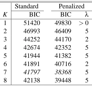
Both standard clustering and penalized clustering selected K=7 by BIC (Table 7), with their predic-tive performances for the test data given in Table 8. The results were close. For penalized clustering, some MPLEs of the cluster-specific mean parameters were exactly zero; their numbers ranged from 36 to 126 in the seven clusters. However, there was no single attribute for which the mean parameter MPLEs were all zero in the seven clusters, hence all the 300 attributes were used in final clustering. This example showed that our penalized clustering performed as well as the standard clustering method for data with none or few non-informative attributes.

Standard Penalized

K BIC BIC λ

1 51420 49830 >0

2 46993 46409 5

3 44252 44170 2

4 42674 42352 5

5 41944 41382 5

6 41891 40716 2

7 41797 38368 5

8 42138 39448 5

Table 7: BIC values for various numbers (K) of clusters in standard and penalized clustering for Hughes’ gene expression data.

Hard classification Soft classification

Standard Penalized Standard Penalized

Truth Pred=1 Pred=2 1 2 1 2 1 2

1 375 31 377 29 265.5 140.5 271.9 134.1

2 111 101 107 105 83.5 128.5 81.4 130.6

Accuracy 0.770 0.780 0.638 0.651

NC(P=300) NSC(P=6) RF SVM

Truth Pred=1 Pred=2 1 2 1 2 1 2

1 313 93 304 102 316 90 362 44

2 61 151 68 144 48 164 81 131

Accuracy 0.751 0.725 0.777 0.798

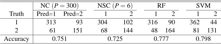
Table 9: Predictions over a separate test data set based on the nearest shrunken centroid without shrinkage (called NC) and with shrinkage (NSC), random forests (RF) and support vector machine (SVM) for Hughes’ gene expression data.

Note that it is in general unfair to compare the predictive performance of a clustering method against that of a classification or supervised learning method; our purpose here was to use the modern classifiers as benchmarks. We used the default setting of R functionrandomForest()for the RF, and usedpamr()andsvm()for the NSC and SVM respectively; for the latter two, a 5-fold cross-validation was used to choose tuning parameters, such as the shrinkage parameter∆in the NSC.

For the NSC, with the selected ∆, only six attributes remained in the final model; however, using all the attributes gave a slightly higher accuracy (Table 9). It was interesting to note that the NSC failed to perform better than either clustering with hard classification. There was some similarity between these two: if we regarded each cluster as a single class, then clustering with hard classification worked in a similar manner as the NSC. Nevertheless, a difference between the two was that, the NSC assumed only one cluster for each class, whereas clustering with hard classification allowed observations of the same class to go to different clusters. Unsurprisingly, the random forests and SVM also performed well for the data.

3.3.2 USING THEDATA WITHADDEDNOISE

It seemed that there were none or few non-informative attributes in the gene expression data for gene function prediction. To mimic other real applications, where a large number of microarray experiments were available, of which however only a fraction are informative, we added 700 noise attributes to the gene expression data. Each noise variable was generated from a standard Normal distribution independent of each other.

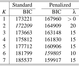
Table 10 summarizes the results of model fitting. By BIC, standard clustering selected K=2 whereas penalized clustering chose K=6. With K=2, standard clustering gave quite bad results for the test data with an accuracy only at about 50% (Table 11), while it performed much better with K=6 (results not shown); in contrast, penalized clustering gave much higher accuracy rates. Note that with many noise attributes, in agreement with that in the previous simulation study, standard clustering probably under-estimated the true number of the clusters of interest at K=2. In addition, a distinct advantage of penalized clustering was that it could correctly identify most non-informative attributes: among the added 700 noise attributes, penalized clustering correctly identified 508 such attributes; in total, 521 attributes whose cluster-specific means were estimated to be 0 for all the clusters in penalized clustering.

Standard Penalized

K BIC BIC λ

1 173221 167960 >0

2 172209 164909 20

3 173663 163148 15

4 175812 161830 15

5 177712 160906 15

6 181799 159805 10

7 185537 159917 15

Table 10: BIC values for various numbers (K) of clusters in standard and penalized clustering for Hughes’ gene expression data with added noise.

Hard classification Soft classification

Standard Penalized Standard Penalized

Truth Pred=1 Pred=2 1 2 1 2 1 2

1 263 143 307 99 203.0 203.0 265.4 140.6

2 149 63 73 139 106.0 106.0 82.2 129.8

Accuracy 0.527 0.722 0.500 0.639

Table 11: Predictions of standard clustering and penalized clustering over a separate test data set for Hughes’ gene expression data with added noise.

NC (P=1000) NSC (P=1) LDA RF SVM

Truth Pred=1 Pred=2 1 2 1 2 1 2 1 2

1 213 193 200 206 275 131 312 94 322 84

2 105 107 111 101 65 147 50 162 57 155

Accuracy 0.518 0.487 0.683 0.767 0.772

why the NSC did not work in this example. One possible explanation was that there were multiple centroids for each class, contrary to the assumption of the NSC that there was only a single one for each class. Hence, we applied linear discriminant analysis (LDA), which imposed an assumption similar to that of the NSC. Although there was a warning message from the R functionlda()(due to P>n), the LDA performed much better than the NSC.

4. Discussion

Penalized likelihood has been widely used in model regularization, particularly for variable selec-tion. A general theory has been laid out, see, for example, Fan and Li (2001), but mainly in the context of regression and classification. We are not aware of any other penalized likelihood ap-proaches to multivariate model-based clustering, which we have studied in this article. In particular, it is confirmed that with the chosen L1 penalty function, it yields a simple thresholding, enabling automatic variable selection. Our numerical examples demonstrate the usefulness of our proposal, especially for “high dimension, low sample size” settings. In particular, our numerical studies suggest the following two points. First, clustering without variable selection may fail to uncover interesting structures underlying the data. Second, best subset selection not only is computationally infeasible for clustering high-dimensional data, but also may fail in small problems. In addition to high computational demand, a key issue with best subset selection is the lack of an appropriate model selection criterion: if a conventional criterion is adopted based on the correctness of a model, because of the existence of many correct models, the criterion will not be useful; for example, any model containing one cluster based on any noise variable or their combinations is correct, but of no interest, in clustering analysis.

The basic idea proposed here is generalizable to semi-supervised learning where some, but not all, observations have class labels. An approach to semi-supervised learning is to conduct clus-tering analysis (i.e., class discovery) simultaneously with supervised learning (i.e., classification) with a mixture model (McLachlan and Peel, 2002). Alexandridis et al. (2004) proposed such a semi-supervised learning approach with an application to tumor classification and class discov-ery. A drawback of their approach was that variable selection had to be taken prior to cluster-ing/classification: they conducted variable selection using either supervised learning or other heuris-tics, then used the selected variables in the subsequent clustering/classification. Pan et al. (2006) ex-tended the penalized likelihood approach discussed here to semi-supervised learning so that variable selection is accomplished simultaneously along with model fitting (i.e., clustering/classification). In particular, their simulation results clearly demonstrated the advantage of simultaneous variable se-lection and model fitting over that of separating variable sese-lection from model fitting.

in model-based clustering, as the use of a common diagonal covariance matrix in the NSC for the same purpose of variable selection for classification. For example, consider an attribute xpwith

dis-tribution N(0,1)or N(0,2)for the two clusters respectively: although its means are equal, because of its different variances in the two clusters, it is still informative to discriminating between the two clusters. It is unclear how to realize automatic variable selection for other more general covariance matrices in penalized model-based clustering. Nevertheless, we acknowledge that it may be desir-able to use more flexible covariance structures, for example, a non-diagonal covariance matrix, in some applications (McLachlan et al., 2003), and more work is needed to explore how to realize variable selection with such a choice in penalized model-based clustering.

In penalized/regularized methods, an important issue is the choice of the penalization param-eter. Although cross-validation and other data-resampling methods can be adopted, due to their high computational cost and possibly sub-optimal performance (Efron, 2004), we have proposed a modified BIC as a model selection criterion. Based on the new results on degrees of freedom in the context of L1-penalized regression (Efron et al., 2004; Zou et al., 2004), we propose counting only non-zero components of the maximum penalized likelihood estimate when calculating the ef-fective number of parameters in BIC. Although it seemed to work well in our numerical examples, theoretical justifications and further evaluations are needed.

Acknowledgments

WP was supported by NIH grant HL65462 and a UM AHC Development grant, XS by NSF grants IIS-0328802 and DMS-0604394. WP thanks Benhuai Xie, Guanghua Xiao and Peng Wei for assis-tance with the gene expression data. The authors thank the two reviewers and the Action Editor for many helpful and constructive comments.

References

R. Alexandridis, S. Lin, and M. Irwin. Class discovery and classification of tumor samples using mixture modeling of gene expression data. Bioinformatics, 20:2546-2552, 2004.

P. J. Bickel, and E. Levina. Some theory for Fisher’s linear discriminant function, “naive Bayes”, and some alternatives when there are many more variables than observations. Bernoulli, 10:989-1010, 2004.

L. Breiman. Random forests. Machine Learning 45:5-32, 2001.

M. P. Brown, W. N. Grundy, D. Lin, N. Cristianini, C. W. Sugnet, T. S. Furey, M. Ares, and D. Haussle. Knowledge-based analysis of microarray gene expression data using support vector ma-chines. Proc Natl Acad Sci USA, 97:262-267, 2000.

W. C. Chang. On using principal components before separating a mixture of two multivariate normal distributions. Applied Statistics, 32:267-275, 1983.

A. P. Dempster, N. M. Laird, and D. B. Rubin. Maximum likelihood from incomplete data via the EM algorithm (with discussion). JRSS-B, 39:1-38, 1977.

B. Efron. The estimation of prediction error: covariance penalties and cross-validation. JASA, 99:619-632, 2004.

B. Efron, T. Hastie T, I. Johnstone I, and R. Tibshirani. Least angle regression. Annals of Statistics, 32:407-499, 2004.

M. Eisen, P. Spellman, P. Brown, and D. Botstein. Cluster analysis and display of genome-wide expression patterns. PNAS, 95:14863-14868, 1998.

J. Fan, and R. Li. Variable selection via nonconcave penalized likelihood and its Oracle properties. JASA, 96:1348-1360, 2001.

C. Fraley, and A. E. Raftery. How many clusters? Which clustering methods? - Answers via model-based cluster analysis. The Computer Journal, 41:578-588, 1998.

C. Fraley, and A. E. Raftery. Model-based clustering, discriminant analysis, and density estimation. Journal of the American Statistical Association, 97:611-631, 2002.

C. Fraley, and A. E. Raftery. Bayesian regularization for normal mixture estimation and model-based clustering. Technical report 486, Dept. of Statistics, University of Washington, 2005.

J. H. Friedman, and J. J. Meulman. Clustering objects on subsets of attributes (with discussion). J. R. Stat. Soc. Ser. B, 66:815-849, 2004.

D. Ghosh D, and A. M. Chinnaiyan. (2002). Mixture modeling of gene expression data from mi-croarray experiments. Bioinformatics, 18:275-286, 2002.

T. R. Golub, D. K. Slonim, P. Tamayo, C. Huard, M. Gaasenbeek, J. P. Mesirov, H. Coller, M. L. Loh, J. R. Downing, M. A. Caligiuri, C. D. Bloomfield, and E. S. Lander. Molecular classification of cancer: class discovery and class prediction by gene expression monitoring. Science, 286:531-537, 1999.

P. J. Green. On use of the EM for penalized likelihood estimation. J. R. Stat. Soc. Ser. B, 52:443-452, 1990.

T. Hastie, R. Tibshirani, and J. Friedman. The Elements of Statistical Learning. Data Mining, Infer-ence, and Prediction. Springer, 2001.

P. D. Hoff. Discussion of ‘Clustering objects on subsets of attributes’ by Friedman and Meulman. J. R. Stat. Soc. Ser. B, 66:845-846, 2004.

P. D. Hoff. Subset clustering of binary sequences, with an application to genomic abnormality data. Biometrics, 61:1027-1036, 2005.

T. R. Hughes, M. J. Marton, A. R. Jones, C. J. Roberts, R. Stoughton, C. D. Armour, H. A. Bennett, E. Coffey, H. Dai, Y. D. He, M. J. Kidd, A. M. King, M. R. Meyer, D. Slade, P. Y. Lum, S. B. Stepaniants, D. D. Shoemaker, D. Gachotte, K. Chakraburtty, J. Simon, M. Bard, and S. H. Friend. Functional Discovery via a Compendium of Expression Profiles. Cell, 102:109-126, 2000.

A. Jasra, C. C. Holmes, and D. A. Stephens. Markov chain Monte Carlo methods and the label switching problem in Bayesian mixture modeling. Statistical Science, 20:50-67, 2005.

S. Kim, M. G. Tadesse, and M. Vannucci. Variable selection in clustering via Dirichlet process mixture models. Biometrika, 93:877-893, 2006.

H. Li, and F. Hong. Cluster-Rasch models for microarray gene expression data. Genome Biology, 2: research0031.1-0031.13, 2001.

J. S. Liu, J. L. Zhang, M. J. Palumbo, C. E. Lawrence. Bayesian clustering with variable and trans-formation selection (with discussion). Bayesian Statistics, 7:249-275, 2003.

O. L. Mangasarian, and E. W. Wild. Feature selection in k-median clustering. Proceedings of SIAM International Conference on Data Mining, Workshop on Clustering High Dimensional Data and its Applications, April 24, 2004, La Buena Vista, FL, pages 23-28.

G. J. McLachlan, R. W. Bean, and D. Peel. A mixture model-based approach to the clustering of microarray expression data. Bioinformatics, 18:413-422, 2002.

G. J. McLachlan, and D. Peel. Finite Mixture Model. New York, John Wiley & Sons, Inc, 2002.

G. J. McLachlan, D. Peel, and R. W. Bean. Modeling high-dimensional data by mixtures of factor analyzers. Computational Statistics and Data Analysis, 41:379-388, 2003.

H. W. Mewes, C. Amid, R. Arnold, D. Frishman, U. Guldener, G. Mannhaupt, M. Munsterkotter, P. Pagel, N. Strack, V. Stumpflen, J. Warfsmann, and A. Ruepp. MIPS: analysis and annotation of proteins from whole genomes. Nucleic Acids Res., 32:D41-D44, 2004.

W. Pan. A comparative review of statistical methods for discovering differentially expressed genes in replicated microarray experiments. Bioinformatics, 12:546-554, 2002.

W. Pan, X. Shen, A. Jiang, and R. P. Hebbel. Semi-supervised learning via penalized mixture model with application to microarray sample classification. Bioinformatics, 22:2388-2395, 2006.

A. E. Raftery. Discussion of “Bayesian clustering with variable and transformation selection” by Liu et al. Bayesian Statistics, 7:266-271, 2003.

A. E. Raftery, and N. Dean. Variable selection for model-based clustering. Journal of the American Statistical Association, 101:168-178, 2006.

S. Richardson, and P. J. Green. On Bayesian analysis of mixtures with an unknown number of components. JRSS-B, 59:731-758, 1997.

X. Shen, and J. Ye. Adaptive model selection. Journal of the American Statistical Association, 97:210-221, 2002.

M. G. Tadesse, N. Sha, and M. Vannucci. Bayesian variable selection in clustering high-dimensional data. Journal of the American Statistical Association, 100:602-617, 2005.

J. G. Thomas, J. M. Olson, S. J. Tapscott, and L. P. Zhao. An efficient and robust statistical modeling approach to discover differentially expressed genes using genomic expression profiles. Genome Research, 11:1227-1236, 2001.

R. Tibshirani. Regression shrinkage and selection via the Lasso. JRSS-B, 58:267-288, 1996.

R. Tibshirani, T. Hastie, B. Narasimhan, and G. Chu. Class prediction by nearest shrunken centroids, with application to DNA microarrays. Statistical Science, 18:104-117, 2003.

V. Vapnik. Statistical Learning Theory. Wiley, 1998.

L. F. Wu, T. R. Hughes, A. P. Davierwala, M. D. Robinson, R. Stoughton, and S. J. Altschuler. Large-scale prediction of saccharomyces cerevisiae gene function using overlapping transcrip-tional clusters. Nature Genetics, 31:255-265, 2002.

G. Xiao, and W. Pan. Gene function prediction by a combined analysis of gene expression data and protein-protein interaction data. Journal of Bioinformatics and Computational Biology, 3:1371-1389, 2005.

K. Y. Yeung, and W. L. Ruzzo. Principal component analysis for clustering gene expression data. Bioinformatics, 17:763-774, 2001.

K. Y. Yeung, C. Fraley, A. Murua, A. E. Raftery, and W. L. Ruzzo. Model-based clustering and data transformations for gene expression data. Bioinformatics, 17:977-987, 2001.

X. Zhou, M. C. Kao, and W. H. Wong. Transitive functional annotation by shortest-path analysis of gene expression data. Proc Natl Acad Sci USA, 99:12783-12788, 2002.