Learning Algorithms for Second-Price Auctions with Reserve

Learning Algorithms for Second-Price Auctions with Reserve

Mehryar Mohri and Andr´es Mu ˜noz Medina Courant Institute of Mathematical Sciences

251 Mercer Street New York, NY, 10012

Editor:Kevin Murphy

Abstract

Second-price auctions with reserve play a critical role in the revenue of modern search engine and popular online sites since the revenue of these companies often directly depends on the outcome of such auctions. The choice of the reserve price is the main mechanism through which the auction revenue can be influenced in these electronic markets. We cast the problem of selecting the reserve price to optimize revenue as a learning problem and present a full theoretical analysis dealing with the complex properties of the corresponding loss function. We further give novel algorithms for solving this problem and report the results of several experi-ments in both synthetic and real-world data demonstrating their effectiveness.

Keywords:Learning Theory, Auctions, Revenue Optimization

1. Introduction

Over the past few years, advertisement has gradually moved away from the traditional printed promotion to the more tailored and directed online publicity. The advantages of online advertisement are clear: since most modern search engine and popular online site companies such as Microsoft, Facebook, Google, eBay, or Amazon may collect information about the users’ behavior, advertisers can better target the population sector for which their brand is intended.

More recently, a new method for selling advertisements has gained momentum. Unlike the standard contracts between publishers and advertisers where some amount of impressions are required to be fulfilled by the publisher, an Ad Exchange works in a way similar to a financial exchange where advertisers bid and compete between each other for an ad slot. The winner then pays the publisher and his ad is displayed.

The design of such auctions and their properties are crucial since they generate a large fraction of the revenue of popular online sites. These questions have motivated extensive research on the topic of auctioning in the last decade or so, particularly in the theoretical computer science and economic theory communities. Much of this work has focused on the analysis of mechanism design, either to prove some useful property of an existing auctioning mechanism, to analyze its computational efficiency, or to search for an optimal revenue maximization truthful mechanism (seeMuthukrishnan(2009) for a good discussion of key research problems related to Ad Exchange and references to a fast growing literature therein).

One particularly important problem is that of determining an auction mechanism that achieves optimal revenue (Muthukrishnan,2009). In the ideal scenario where the valuation of the bidders is drawn i.i.d. from a given distribution, this is known to be achievable (see for example (Myerson, 1981)). But, even good approximations of such distributions are not known in practice. Game theoretical approaches to the design of auctions have given a series of interesting results including (Riley and Samuelson,1981;Milgrom and Weber, 1982;Myerson,1981;Nisan et al.,2007), all of them based on some assumptions about the distribution of the bidders, e.g., the monotone hazard rate assumption.

bidders bid exactly what they are willing to pay. It is clear that the revenue of the publisher depends greatly on how the reserve price is set: if set too low, the winner of the auction might end up paying only a small amount, even if his bid was high; on the other hand, if it is set too high, then bidders may not bid higher than the reserve price and the ad slot will not be sold.

We propose a learning approach to the problem of determining the reserve price to optimize revenue in such auctions. The general idea is to leverage the information gained from past auctions to predict a beneficial reserve price. Since every transaction on an Exchange is logged, it is natural to seek to exploit that data. This could be used to estimate the probability distribution of the bidders, which can then be used indirectly to come up with the optimal reserve price (Myerson,1981;Ostrovsky and Schwarz,2011). Instead, we will seek a discriminative method making use of the loss function related to the problem and taking advantage of existing user features.

Learning methods have been used in the past for the related problems of designing incentive-compatible auction mechanisms (Balcan et al.,2008;Blum et al.,2004), for algorithmic bidding (Langford et al.,2010; Amin et al.,2012), and even for predicting bid landscapes (Cui et al.,2011). Another closely related problem for which machine learning solutions have been proposed is that of revenue optimization for sponsored search ads and click-through rate predictions (Zhu et al.,2009;He et al.,2013;Devanur and Kakade,2009). But, to our knowledge, no prior work has used historical data in combination with user features for the sole purpose of revenue optimization in this context. In fact, the only publications we are aware of that are directly related to our objective are (Ostrovsky and Schwarz,2011) and (Cesa-Bianchi et al.,2013), which considers a more general case than (Ostrovsky and Schwarz,2011).

The scenario studied byCesa-Bianchi et al.(2013) is that of censored information, which motivates their use of a regret minimization algorithm to optimize the revenue of the seller. Our analysis assumes instead access to full information. We argue that this is a more realistic scenario since most companies do have access to the full historical data. The learning scenario we consider is also more general since it includes the use of features, as is standard in supervised learning. Since user information is communicated to advertisers and bids are made based on that information, it is only natural to include user features in the formulation of the learning problem. A special case of our analysis coincides with the no-feature scenario considered by Cesa-Bianchi et al.(2013), assuming full information. But, our results further extend those of this paper even in that scenario. In particular, we present anO(mlogm)algorithm for solving a key optimization problem used as a subroutine by these authors, for which they do not seem to give an algorithm. We also do not assume that buyers’ bids are sampled i.i.d. from a common distribution. Instead, we only assume that the full outcome of each auction is independent and identically distributed. This subtle distinction makes our scenario closer to reality as it is unlikely for all bidders to follow the same underlying value distribution. Moreover, even though our scenario does not take into account a possible strategic behavior of bidders between rounds, it allows for bidders to be correlated, which is common in practice.

This paper is organized as follows: in Section2, we describe the setup and give a formal description of the learning problem. We discuss the relations between the scenario we consider and previous work on learning in auctions in Section3. In particular, we show that, unlike previous work, our problem can be cast as that of minimizing the expected value of a loss function, which is a standard learning problem. Unlike most work in this field, however, the loss function naturally associated to this problem does not admit favorable properties such as convexity or Lipschitz continuity. In fact the loss function is discontinuous. Therefore, the theoretical and algorithmic analysis of this problem raises several non-trivial technical issues. Nevertheless, we use a decomposition of the loss to derive generalization bounds for this problem (see Section4). These bounds suggest the use of structural risk minimization to determine a learning solution benefiting from strong guarantees. This, however, poses a new challenge: solving a highly non-convex optimization problem. Similar algorithmic problems have been of course previously encountered in the learning literature, most notably when seeking to minimize a regularized empirical0-1loss in binary classification. A standard method in machine learning for dealing with such issues consists of resorting to a convex surrogate loss (such as the hinge loss commonly used in linear classification). However, we show in Section4.2that no convex loss function is calibrated for the natural loss function for this problem. That is, minimizing a convex surrogate could be detrimental to learning. This fact is further empirically verified in Section6.

of the hypothesis set. This leads to an optimization problem which, albeit non-convex, admits a favorable decomposition as a difference of two convex functions (programming). Thus, we suggest using the DC-programming algorithm (DCA) introduced byTao and An(1998) to solve our optimization problem. This algorithm admits favorable convergence guarantees to alocal minimum. To further improve upon DCA, we propose a combinatorial algorithm to cycle through different local minima with the guarantee of reducing the objective function at every iteration. Finally, in Section6, we show that our algorithm outperforms several different baselines in various synthetic and real-world revenue optimization tasks.

2. Setup

We start with the description of the problem and our formulation of the learning setup. We study second-price auctions with reserve, the type of auctions adopted in many Ad Exchanges. In such auctions, the bidders submit their bids simultaneously and the winner, if any, pays the maximum of the value of the second-place bid and a reserve pricerset by the seller. This type of auctions benefits from the same truthfulness property as second-price auctions (or Vickrey auctions)Vickrey(1961): truthful bidding can be shown to be a dominant strategy in such auctions. The choice of the reserve priceris the only mechanism through which the seller can influence the auction revenue. Its choice is thus critical: if set too low, the amount paid by the winner could be too small; if set too high, the ad slot could be lost. How can we select the reserve price to optimize revenue?

We consider the problem of learning to set the reserve prices to optimize revenue in second-price auctions with reserve. The outcome of an auction can be encoded by the highest and second-highest bids which we denote by a vectorb = (b(1), b(2)) ∈ B ⊂ R2+. We will assume that there exists an upper boundM ∈ (0,+∞)for the bids:sup_b∈Bb(1)=M. For a given reserve pricerand bid pairb, by definition, the revenue

of an auction is given by

Revenue(r,b) =b(2)1r<b(2)+r1_b(2)_≤r≤b(1).

We consider the general scenario where a feature vectorx ∈ X ⊂RN is associated with each auction. In

the auction theory literature, this feature vector is commonly referred to aspublic information. In the context of online advertisement, this could be for example information about the user’s location, gender or age. The learning problem can thus be formulated as that of selecting out of a hypothesis setHof functions mapping

XtoRa hypothesishwith high expected revenue

E

(x,b)∼D[Revenue(h(x),b)], (1)

whereDis an unknown distribution according to which pairs(x,b)are drawn. Instead of the revenue, we will consider a loss functionLdefined for all(r,b)byL(r,b) =−Revenue(r,b), and will equivalently seek a hypothesishwith small expected lossL(h) := E(x,b)∼D[L(h(x),b)]. As in standard supervised learning

scenarios, we assume access to a training sampleS = ((x1,b1), . . . ,(xm,bm))of sizem≥1drawn i.i.d.

according toD. We will denote byLbS(h)the empirical lossLbS(h) = _m1 Pm_i=1L(h(xi,bi)). Notice that

we only assume that the auction outcomes are i.i.d. and not that bidders are independent of each other with the same underlying bid distribution, as in some previous work (Cesa-Bianchi et al., 2013;Ostrovsky and Schwarz,2011). In the next sections, we will present a detailed study of this learning problem, starting with a review of the related literature.

3. Previous work

A step further in the design of optimal pricing strategies was proposed byBalcan et al.(2008). One of the problems considered by the authors was that of setting prices fornbuyers in a posted-price auction as a function of their public information. Unlike the on-line scenario ofBlum et al.(2004),Balcan et al.(2008) considered a batch scenario where all buyers are known in advance. However, the comparison class considered was no longer that of simple fixed-price strategies but functions mapping public information to prices. This makes the problem more challenging and closer to the scenario we consider. The authors showed that finding a(1 +)-optimal truthful mechanism is equivalent to finding an algorithm to optimize the empirical risk associated to the loss function we consider (in the caseb(2)≡0). There are multiple connections between this work and our results. In particular, the authors pointed out that the discontinuity and asymmetry of the loss function presented several challenges to their analysis. We will see that, in fact, the same problems appear in the derivation of our learning guarantees. But, we will present an algorithm for minimizing the empirical risk which was a crucial element missing in their results.

A different line of work byCui et al.(2011) focused on predicting the highest bid of a second-price auction. To estimate the distribution of the highest bid, the authors partitioned the space of advertisers based on their campaign objectives and estimated the distribution for each partition. Within each partition, the distribution of the highest bid was modeled as a mixture of log-normal distributions where the means and standard deviations of the mixtures were estimated as a function of the data features. While it may seem natural to seek to predict the highest bid, we show that this is not necessary and that accurate predictions of the highest bid do not necessarily translate into algorithms achieving large revenue (see Section6).

As already mentioned, the closest previous work to ours is that ofCesa-Bianchi et al.(2013), who studied the problem of directly optimizing the revenue under a partial information setting where the learner can only observe the value of the second-highest bid, if it is higher than the reserve price. In particular, the highest bid remains unknown to the learner. This is a natural scenario for auctions such as those of eBay where only the price at which an object is sold is reported. To do so, the authors expressed the expected revenue in terms of the quantityq(t) =_P[b(2)_{> t]}

. This can be done as follows:

E

b[Revenue(r,b)] =bE(2)[b (2)

1r<b(2)] +rP[b(2)≤r≤b(1)] (2)

= Z +∞

0

P[b(2)1r<b(2)> t]dt+rP[b(2)≤r≤b(1)]

= Z r

0

P[r < b(2)]dt+ Z ∞

r

P[b(2)> t]dt+rP[b(2)≤r≤b(1)]

= Z ∞

r

P[b(2)> t]dt+r(P[b(2)> r] + 1−P[b(2)> r]−P[b(1)< r])

= Z ∞

r

P[b(2)> t]dt+rP[b(1)≥r].

The main observation ofCesa-Bianchi et al.(2013) was that the quantity q(t)can be estimated from the observed outcomes of previous auctions. Furthermore, if the buyers’ bids are i.i.d., then, one can express

P[b(1) ≥r]as a function of the estimated value ofq(r). This implies that the right-hand side of (2) can be

accurately estimated and therefore an optimal reserve price can be selected. Their algorithm makes calls to a procedure that maximizes the empirical revenue. The authors, however, did not describe an algorithm for that maximization. A by-product of our work is an efficient algorithm for that procedure. The guarantees of Cesa-Bianchi et al.(2013) are similar to those presented in the next section in the special case of learning without features. However, our derivation is different since we consider a batch scenario whileCesa-Bianchi et al.(2013) treated an online setup for which they presented regret guarantees.

4. Learning Guarantees

0 1 2 3 4 5 6 7 -5

-4 -3 -2 -1 0

b

b

−

b

(2)

0 1 2 3 4 5 6 7

-5 -4 -3 -2 -1 0

b

b

−

b

(2)

0 1 2 3 4 5 6 7

-1 0 1 2 3 4

b

(a) (b)

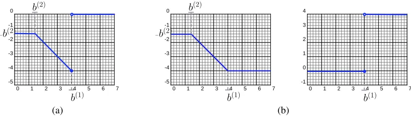
Figure 1: (a) Plot of the loss functionr_7→L(r,b)for fixed values ofb(1)_andb(2)_{; (b) Functionsl} 1on the

left andl2on the right.

4.1 Generalization bound

To analyze the complexity of the family of functionsLHmappingX × BtoRdefined by

LH={(x,b)7→L(h(x),b) :h∈H},

we decomposeLas a sum of two loss functionsl1andl2with more favorable properties thanL. We have

L=l1+l2withl1andl2defined for all(r,b)∈R× Bby

l1(r,b) =−b(2)1r<b(2)−r1_b(2)_≤r≤b(1)−b(1)1_r>b(1)

l2(r,b) =b(1)1r>b(1).

These functions are shown in Figure1(b). Note that, for a fixedb, the functionr7→l1(r,b)is1-Lipschitz since the slope of the lines defining the function is at most1. We will consider the corresponding families of loss functions:l1H ={(x,b)7→l1(h(x),b) :h∈H}andl2H={(x,b)7→l2(h(x),b) :h∈H}and use the notion of pseudo-dimension as well as those of empirical and average Rademacher complexity to measure their complexities. The pseudo-dimension is a standard complexity measure (Pollard,1984) extending the notion of VC-dimension to real-valued functions (see alsoMohri et al.(2012)). For a family of functionsG

and finite sampleS= (z1, . . . , zm)of sizem, the empirical Rademacher complexity is defined byRbS(G) =

Eσsupg∈G

1

m

Pm

i=1σig(zi)

, whereσ= (σ1, . . . , σm)>, withσis independent uniform random variables

taking values in{−1,+1}. The Rademacher complexity ofGis defined asRm(G) =ES∼Dm[RbS(G)].

To bound the complexity ofLH, we will first bound the complexity of the family of loss functionsl1Hand

l2H. Sincel1is1-Lipschitz, the complexity of the classl1Hcan be readily bounded by that ofH, as shown

by the following proposition.

Proposition 1 For any sampleS = ((x1,b1), . . . ,(xm,bm)), the empirical Rademacher complexity ofl1H can be

bounded as follows:

b

RS(l1H)≤RbS(H).

Proof By definition of the empirical Rademacher complexity, we can write

b

RS(l1H) =

1 mEσ

" sup

h∈H m

X

i=1

σil1(h(xi),bi)

# = 1

mEσ

" sup

h∈H m

X

i=1

σi(ψi◦h)(xi)

#

,

where, for all i ∈ [1, m], ψi is the function defined by ψi: r 7→ l1(r,bi). For anyi ∈ [1, m], ψi is

1-Lipschitz, thus, by the contraction lemma of AppendixA(Lemma14), the following inequality holds:

b

RS(l1H)≤

1 mEσ

" sup

h∈H m

X

i=1

σih(xi)

#

=RbS(H),

which completes the proof.

As shown by the following proposition, the complexity ofl2H can be bounded in terms of the

Proposition 2 Letd=Pdim(H)denote the pseudo-dimension ofH, then, for any sampleS= ((x1,b1), . . . ,(xm,bm)),

the empirical Rademacher complexity ofl2Hcan be bounded as follows:

b

RS(l2H)≤M

r

2dlogem d

m .

Proof By definition of the empirical Rademacher complexity, we can write

b

RS(l2H) =

1 mEσ

" sup

h∈H m

X

i=1

σib(1)i 1h(xi)>b(1)i #

= 1 mEσ

" sup

h∈H m

X

i=1

σiΨi(1_h(x

i)>b(1)i )

#

,

where, for alli∈ [1, m],Ψiis theM-Lipschitz functionx7→ b(1)_i x. Thus, by Lemma14combined with

Massart’s lemma (see for exampleMohri et al.(2012)), we can write

b

RS(l2H)≤

M m Eσ

" sup

h∈H m

X

i=1

σi1

h(xi)>b(1)i #

≤M

r

2d0_logem d0

m ,

whered0 = VCdim({(x,b) 7→ 1h(x)−b(1)_>0: (x,b) ∈ X × B}). Since the second bid componentb(2) plays no role in this definition,d0coincides with VCdim({(x, b(1))7→1h(x)−b(1)_>0: (x, b(1))∈ X × B1}), whereB1is the projection ofB ⊆R2onto its first component, and is upper-bounded by VCdim({(x, t)7→

1h(x)−t>0: (x, t)∈ X ×R}), that is, the pseudo-dimension ofH.

Propositions1and2can be used to derive the following generalization bound for the learning problem we consider.

Theorem 3 For anyδ >0, with probability at least1−δover the draw of an i.i.d. sampleSof sizem, the following inequality holds for allh∈H:

L(h)≤LbS(h) + 2Rm(H) + 2M

r

2dlogem d

m +M

s log1

δ

2m .

ProofBy a standard property of the Rademacher complexity, sinceL=l1+l2, the following inequality holds: Rm(LH)≤Rm(l1H) +Rm(l2H). Thus, in view of Propositions1and2, the Rademacher complexity of

LHcan be bounded via

Rm(LH)≤Rm(H) +M

r

2dlogem_d

m .

The result then follows by the application of a standard Rademacher complexity bound (Koltchinskii and Panchenko,2002).

This learning bound invites us to consider an algorithm seekingh ∈ Hto minimize the empirical loss

b

LS(h), while controlling the complexity (Rademacher complexity and pseudo-dimension) of the hypothesis

setH. In the following section, we discuss the computational problem of minimizing the empirical loss and suggest the use of a surrogate loss leading to a more tractable problem.

4.2 Surrogate Loss

As previously mentioned, the loss functionLdoes not admit most properties of traditional loss functions used in machine learning: for any fixedb,L(·,b)is not differentiable (at two points), it is not convex nor Lipschitz, and in fact it is discontinuous. For any fixedb,L(·,b)is quasi-convex,1_{a property that is often}

desirable since there exist several solutions for quasi-convex optimization problems. However, in general, a sum of quasi-convex functions, such as the sumPm

i=1L(·,bi)appearing in the definition of the empirical

loss, is not quasi-convex and a fortiori not convex.2 In general, such a sum may admit exponentially many local minima. This leads us to seek a surrogate loss function with more favorable optimization properties.

1. A functionf:R→Ris said to bequasi-convexif for anyα∈Rthe sub-level set{x:f(x)≤α}is convex.

0 1 2 3 4 5 6 7

-5 -4 -3 -2 -1 0

1 b2

b1

(a) (b)

Figure 2: (a) Piecewise linear convex surrogate loss Lp. (b) Comparison of the sum of real losses

Pm

i=1L(·,bi)for m = 500with the sum of convex surrogate losses. Note that the minimizers are significantly different.

A standard method in machine learning consists of replacing the loss functionLwith a convex upper bound (Bartlett et al.,2006). A natural candidate in our case is the piecewise linear functionLpshown in

Figure2(a). While this is a convex loss function, and thus convenient for optimization, it is not calibrated. That is, it is possible forrp∈argminEb[Lp(r,b)]to have a large expected true loss. Therefore, it does not

provide us with a useful surrogate. The calibration problem is illustrated by Figure2(b) in dimension one, where the true objective function to be minimizedPm

i=1L(r,bi)is compared with the sum of the surrogate

losses. The next theorem shows that this problem affectsanynon-constant convex surrogate. It is expressed in terms of the lossLe:_R×_R+→Rdefined byLe(r, b) =−r1r≤b, which coincides withLwhen the second

bid is0.

Definition 4 We say that a functionLc: [0, M]×[0, M]→Risconsistent withLeif, for any distributionD, there exists a minimizerr∗∈argminrEb∼D[Lc(r, b)]such thatr∗∈argminrEb∼D[Le(r, b)].

Definition 5 We say that a sequence of functions(Ln)n∈Nmapping[0, M]×[0, M]toRisweakly consistent withLe if there exists a sequence(rn)n∈NinRwithrn∈argminrEb∼D[Ln(r, b)]for alln∈Nsuch thatlimn→+∞rn=r∗

withr∗∈argminEb∼D[Le(r, b)].

Proposition 6 (Convex surrogates) LetLc: [0, M]×[0, M] →Rbe a bounded function, convex with respect to its first argument. IfLcis consistent withLe, thenLc(·, b)is constant for anyb∈[0, M].

Proof The idea behind the proof is the following: for any two bidsb1< b2, there exists a distributionDwith support{b1, b2}such thatEb∼D[Le(r, b)]is minimized at bothr=b1andr=b2. We show this implies that

Eb∼D[Lc(r, b)]must attain a minimum at both points too. By convexity ofLc, it follows thatEb∼D[Lc(r, b)]

must be constant on the interval[b1, b2]. The main part of the proof will be showing that this implies that the functionLc(·, b1)must also be constant on the interval[b1, b2]. Finally, since the value ofb2was chosen arbitrarily, it will follow thatLc(·, b1)is constant.

Let0< b1 < b2 < Mand, for anyµ ∈[0,1], letDµdenote the probability distribution with support

included in{b1, b2}defined byDµ(b1) =µand letEµdenote the expectation with respect to this distribution.

A straightforward calculation shows that the unique minimizer ofEµ[Le(r, b)]is given byb2ifµ > b2_b−b1 2 and byb1ifµ < b2_b−b1

2 . Therefore, ifFµ(r) =Eµ[Lc(r, b)], it must be the case thatb2is a minimizer ofFµfor µ >b2−b1

b2 andb1is a minimizer ofFµforµ <

b2−b1

b2 .

For a convex functionf:R → R, we denote byf−its left-derivative and byf+ its right-derivative,

which are guaranteed to exist. We will also denote here, for anyb∈R, byg−(·, b)andg+_{(·, b)}

ofb1andb2, the following inequalities hold:

0≥Fµ−(b2) =µL−c(b2, b1) + (1−µ)L−c(b2, b2) forµ >

b2−b1

b2

, (3)

0≤Fµ+(b1)≤F

−

µ(b2) forµ <

b2−b1

b2

, (4)

where the second inequality in (4) holds by convexity ofFµand the fact thatb1 < b2. By settingµ= b2_b−b1 2 , it follows from inequalities (3) and (4) thatFµ−(b2) = 0andFµ+(b1) = 0. By convexity ofFµ, it follows that

Fµis constant on the interval(b1, b2). We now show this may only happen ifLc(·, b1)is also constant. By rearranging terms in (3) and plugging in the expression ofµ, we obtain the equivalent condition

(b2−b1)L

−

c(b2, b1) =−b1L

−

c(b2, b2).

SinceLcis a bounded function, it follows thatL−c(b2, b1)is bounded for anyb1, b2 ∈(0, M), therefore as

b1 →b2we must haveb2L−c(b2, b2) = 0, which impliesL−c(b2, b2) = 0for allb2 >0. In view of this, inequality (3) may only be satisfied ifL−c(b2, b1)≤0. However, the convexity ofLcimpliesL−c(b2, b1)≥

L−c(b1, b1) = 0. Therefore,L−c(b2, b1) = 0must hold for allb2 > b1 >0. Similarly, by definition ofFµ,

the first inequality in (4) implies

µL+c(b1, b1) + (1−µ)L+c(b1, b2)≥0. (5)

Nevertheless, for anyb2 > b1 we have0 = Lc−(b1, b1) ≤ L+c(b1, b1) ≤L−c(b2, b1) = 0. Consequently,

L+

c(b1, b1) = 0for allb1 >0. Furthermore,L+c(b1, b2)≤L+c(b2, b2) = 0. Therefore, for inequality (5) to be satisfied, we must haveL+c(b1, b2) = 0for allb1< b2.

Thus far, we have shown that for anyb >0, ifr≥b, thenL−c(r, b) = 0, whileL

+

c(r, b) = 0forr≤b.

A simple convexity argument shows thatLc(·, b)is then differentiable andL0c(r, b) = 0for allr∈(0, M),

which in turn implies thatLc(·, b)is a constant function.

The result of the previous proposition can be considerably strengthened, as shown by the following theorem. As in the proof of the previous proposition, to simplify the notation, for anyb∈R, we will denote byg0(·, b)

the derivative of a differentiable functiong(·, b).

Theorem 7 Let(Ln)n∈Ndenote a sequence of functions mapping[0, M]×[0, M]toRthat are convex and differentiable

with respect to their first argument and satisfy the following conditions: • supb∈[0,M],n∈Nmax(|L

0

n(0, b)|,|L0n(M, b)|=K <∞;

• (Ln)nis weakly consistent withLe; • Ln(0, b) = 0for alln∈Nand for allb.

If the sequence(Ln)nconverges pointwise to a functionLc, thenLn(·, b)converges uniformly toLc(·, b)≡0.

We defer the proof of this theorem to AppendixBand present here only a sketch of the proof. We first show that the convexity of the functionsLn implies that the convergence toLc must be uniform and thatLcis

convex with respect to its first argument. This fact and the weak consistency of the sequenceLnwill then

imply thatLcis consistent withLeand therefore must be constant by Proposition6.

The theorem just presented shows that even a weakly consistent sequence of convex losses is uniformly close to a constant function and therefore not helpful to tackle the learning task we consider. This suggests searching for surrogate losses that admit weaker regularity assumptions such as Lipschitz continuity.

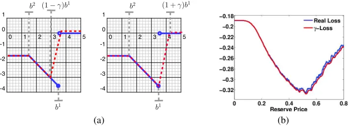
Perhaps, the most natural surrogate loss function is thenLγ, an upper bound onLdefined for allγ >0

by:

Lγ(r,b) =−b(2)1r≤b(2)−r1

b(2)<r≤ (1−γ)b(1)∨b(2)

+1−γ

γ ∨

b(2)

b(1)_−b(2)

(r−b(1))1 _(1−γ)b(1)∨b(2)_<r≤b(1),

0 1 2 3 4 5

-4 -3 -2 -1 0 1

b2 _(1−γ)b1

b1

0 1 2 3 4 5

-4 -3 -2 -1 0 1

b2 _{(1 +γ)b}1

b1

(a) (b)

Figure 3: (a) Comparison of the true lossLwith surrogate lossLγ on the left and surrogate lossLγ on the right, forγ= 0.1. (b) Comparison ofP500

i=1L(r,bi)andP

500

i=1Lγ(r,bi)

upper bound onLin the most critical region, that is around the minimum of the lossL. Thus, instead, we will consider, for anyγ >0, the loss functionLγdefined as follows:

Lγ(r,b) =−b(2)1r≤b(2)−r1_b(2)_<r≤b(1)+

1

γ(r−(1 +γ)b

(1)

)1b(1)_<r≤(1+γ)b(1), (6)

whose plot is shown in Figure3(a).3 A comparison between the sum ofL-losses and the sum ofLγ-losses

is shown in Figure3(b). Observe that the fit is considerably better than that of the piecewise linear convex surrogate loss shown in Figure2(b). A possible concern associated with the loss functionLγis that it is a lower

bound forL. One might think then that minimizing it would not lead to an informative solution. However, we argue that this problem arises significantly with upper bounding losses such as the convex surrogate, which we showed not to lead to a useful minimizer, orLγ, which is a poor approximation ofLnear its

minimum. By matching the original loss Lin the region of interest, around the minimal value, the loss functionLγleads to more informative solutions for this problem. In fact, we show that that the expected loss

Lγ(h) : =Ex,b[Lγ(h)]admits a minimizer close to the minimizer ofL(h). SinceLγ →Lasγ→0, this

result may seem trivial. However, this convergence is not uniform and therefore calibration is not guaranteed.

Theorem 8 LetHbe a closed, convex subset of a linear space of functions containing0. Then, the following inequality holds for allγ≥0:

L(h∗γ)− Lγ(h

∗

γ)≤γM.

Notice that, sinceL ≥Lγfor allγ ≥0, the theorem implies thatlimγ→0L(h∗γ) =L(h

∗

). Indeed, leth∗

denote the best-in-class hypothesis for the loss functionL. Then, the following straightforward inequalities hold:

L(h∗)≤ L(h∗γ)

≤ Lγ(h∗γ) +γM

≤ Lγ(h

∗

) +γM≤ L(h∗) +γM.

By letting γ → 0, we see thatL(h∗γ) → L(h

∗

). This is a remarkable result as it not only provides a convergence guarantee, but it also gives us an explicit rate of convergence. We will later exploit this fact to derive an optimal choice forγ.

The proof of Theorem8is based on the following partitioning ofX × Bin four regions whereLγ is

defined as an affine function:

I1={(x,b)|h

∗

γ(x)≤b

(2)

} I2={(x,b)|h

∗

γ(x)∈(b

(2)

, b(1)]}

I3={(x,b)|h∗γ(x)∈(b

(1)

,(1 +γ)b(1)]} I4={(x,b)|h∗γ(x)>(1 +γ)b

(1)

},

Notice thatLγandLdiffer only onI3. Therefore, we only need to bound the measure of this set which can

be done as in Lemma15(see AppendixC).

Proof[Theorem8]. We can express the difference as

E x,b

h

L(h∗γ(x),b)−Lγ(h

∗

γ(x),b)

i =

4

X

k=1

E x,b

h

(L(h∗γ(x),b)−Lγ(h

∗

γ(x),b))1Ik(x,b) i

= E x,b

h

(L(h∗γ(x),b)−Lγ(h∗γ(x),b))1I3(x,b)

i

= E x,b

h1

γ((1 +γ)b

(1)

−h∗γ(x))1I3(x,b))

i

. (7)

Furthermore, for(x,b)∈I3, we know thatb(1)_{< h}∗

γ(x). Thus, we can bound (7) byEx,b[hγ∗(x)1I3(x,b)], which, by Lemma15in AppendixC, is upper bounded byγEx,b

h

h∗γ(x)1I2(x,b)

. Thus, the following inequalities hold:

E x,b

h

L(h∗γ(x),b)

i − E

x,b h

Lγ(h

∗

γ(x),b)

i ≤γ E

x,b h

h∗γ(x)1I2(x,b)

i ≤γ E

x,b h

b(1)1I2(x,b)

i ≤γM,

using the fact thath∗γ(x)≤b(1)for(x,b)∈I2.

The1/γ-Lipschitzness ofLγcan be used to prove the following generalization bound.

Theorem 9 Fixγ∈(0,1]and letSdenote a sample of sizem. Then, for anyδ >0, with probability at least1−δover the choice of the sampleS, for allh∈H, the following holds:

Lγ(h)≤Lbγ(h) +

2

γRm(H) +M

s log1

δ

2m . (8)

Proof LetLγ,Hdenote the family of functions{(x,b)→Lγ(h(x), b) :h∈H}. The loss functionLγis_γ1

-Lipschitz since the slope of the lines defining it is at most1

γ. Thus, using the contraction lemma (Lemma14)

as in the proof of Proposition1, givesRm(Lγ,H)≤ 1_γRm(H). The application of a standard Rademacher

complexity bound to the family of functionsLγ,Hthen shows that for anyδ > 0, with probability at least

1−δ, for anyh∈H, the following holds:

Lγ(h)≤Lbγ(h) +

2

γRm(H) +M

s log1

δ

2m .

We conclude this section by showing thatLγadmits a stronger form of consistency. More precisely, we prove

that the generalization error of the best-in-class hypothesisL∗

:=L(h∗)can be lower bounded in terms of that of the empirical minimizer ofLγ,bhγ: = argminh∈HLbγ(h).

Theorem 10 LetM = supb∈Bb

(1)

and letHbe a hypothesis set with pseudo-dimensiond=Pdim(H).Then, for any

δ >0and a fixed value ofγ >0, with probability at least1−δover the choice of a sampleSof sizem, the following inequality holds:

L∗≤ L(bhγ)≤ L∗+

2γ+ 2

γ Rm(H) +γM+ 2M

r

2dlogm_d

m + 2M

s log2_δ

2m .

Proof By Theorem3, with probability at least1−δ/2, the following holds:

L(bhγ)≤LbS(bhγ) + 2Rm(H) + 2M

r

2dlogm_d

m +M

s log2_δ

−a(1)

b(2)

−a(2)r

b(1) a(3)_r

−a(4)

(1 +η)b(1) b(2)i b

(1)

i nk nk₊₁

(1 +η)b(1)i

Vi(nk,bi) =−a(2)i nk Vi(nk₊₁,bi) =−a(2)i nk₊₁

(a) (b)

Figure 4: (a) Prototypical v-function. (b) Illustration of the fact that the definition ofVi(r,bi) does not change on an interval[nk, nk+1].

Applying Lemma 15 with the empirical distribution induced by the sample, we can bound LbS(bhγ) by

b

Lγ(bhγ) +γM. The first term of the previous expression is less thanLbγ(h∗γ)by definition ofbhγ.

More-over, the same analysis used in the proof of Theorem9shows that with probability1−δ/2,

b

Lγ(h∗γ)≤ Lγ(h∗γ) +

2

γRm(H) +M

s log2_δ

2m .

Finally, by definition ofh∗γ and using the fact thatLis an upper bound on Lγ, we can writeLγ(h∗γ) ≤

Lγ(h∗)≤ L(h∗). Thus,

b

LS(bhγ)≤ L(h

∗ ) +2

γRm(H) +M

s log2

δ

2m +γM.

Replacing this inequality in (9) and applying the union bound yields the result.

This bound can be extended to hold uniformly over allγat the price of a term inO q

log log_√ 2γ1

m

. Thus, for

appropriate choices ofγas a function ofm(for instanceγ= 1/m1/4) we can guarantee the convergence of

L(bhγ)toL∗, a stronger form of consistency (See AppendixC).

These results are reminiscent of the standard margin bounds withγ playing the role of a margin. The situation here is however somewhat different. Our learning bounds suggest, for a fixedγ ∈ (0,1], to seek a hypothesishminimizing the empirical lossLbγ(h) while controlling a complexity term upper bounding

Rm(H), which in the case of a family of linear hypotheses could bekhk2Kfor some PSD kernelK. Since

the bound can hold uniformly for allγ, we can use it to selectγ out of a finite set of possible grid search values. Alternatively,γcan be set via cross-validation. In the next section, we present algorithms for solving this regularized empirical risk minimization problem.

5. Algorithms

In this section, we show how to minimize the empirical risk under two regimes: first we analyze the no-feature scenario considered inCesa-Bianchi et al.(2013) and then we present an algorithm to solve the more general feature-based revenue optimization problem.

5.1 No-Feature Case

We now present a general algorithm to optimize sums of functions similar toLγorLin the one-dimensional

case.

witha(1) > 0andη > 0constants anda(2), a(3), a(4) defined bya(1) = ηa(3)b(2), a(2) = ηa(3), and a(4) = a(3)_{(1 +η)b}(1)

.

Figure4(a) illustrates this family of loss functions. Av-function is a generalization ofLγandL. Indeed, any

v-functionV satisfiesV(r,b)≤0and attains its minimum atb(1). Finally, as can be seen straightforwardly from Figure3,Lγis av-function for anyγ >0. We consider the following general problem of minimizing a

sum ofv-functions:

min

r≥0 F(r) :=

m

X

i=1

Vi(r,bi). (10)

Observe that this is not a trivial problem since, for any fixedbi,Vi(·,bi)is non-convex and that, in general,

a sum ofmsuch functions may admit many local minima. Of course, we can seek a solution that is-close to the optimal reserve via a grid search over pointsri=i. However, the guarantees for that algorithm would

depend on the continuity of the function. In particular, this algorithm might fail for the lossL. Instead, we exploit the particular structure of av-function to exactly minimizeF. The following proposition, which is proven in AppendixD, shows that the minimum is attained at one of the highest bids, which matches the intuition. Notice that for the loss functionLthis is immediate since ifris not a highest bid, one can raise the reserve price without increasing any of the component losses.

Proposition 12 Problem(10)admits a solutionr∗that satisfiesr∗=b(1)i for somei∈[1, m].

Problem (10) can thus be reduced to examining the value of the function for the m argumentsb(1)_i ,

i ∈ [1, m]. This yields a straightforward method for solving the optimization which consists of comput-ingF(b(1)i )for alliand taking the minimum. But, since the computation of eachF(b

(1)

i )takesO(m), the

overall computational cost is inO(m2_{), which can be prohibitive for even moderately large values ofm.} Instead, we present a combinatorial algorithm to solve the optimization problem (10) inO(mlogm). Let

N =S

i{b

(1)

i , b

(2)

i ,(1 +η)b

(1)

i }denote the set of allboundary pointsassociated with the functionsV(·,bi).

The algorithm proceeds as follows: first, sort the setN to obtain the ordered sequence(n1, . . . , n3m), which

can be achieved inO(mlogm)using a comparison-based sorting algorithm. Next, evaluateF(n1)and com-puteF(nk+1)fromF(nk)for allk.

The main idea of the algorithm is the following: since the definition ofVi(·, bi) can only change at

boundary points (see also Figure4(b)), computingF(nk+1)fromF(nk)can be achieved in constant time.

Indeed, since betweennkandnk+1there are only two boundary points, we can computeV(nk+1,bi)from

V(nk,bi)by calculatingV for only two values ofbi, which can be done in constant time. We now give a

more detailed description and proof of correctness of our algorithm.

Proposition 13 There exists an algorithm to solve the optimization problem(10)inO(mlogm).

Proof The pseudocode of the algorithm is given in Algorithm1, wherea(1)_i , ..., a(4)_i denote the parameters defining the functionsVi(r,bi). We will prove that, after running Algorithm1, we can computeF(nj)in

constant time using:

F(nj) =c(1)j +c

(2)

j nj+c(3)j nj+c(4)j . (11)

This holds trivially forn1since by definitionn1 ≤b(2)i for alliand thereforeF(n1) =−Pm_i=1a(1)i . Now,

assume that (11) holds forj, we prove that it must also hold forj+ 1. Supposenj =b

(2)

i for somei(the

casesnj =b(1)i andnj= (1 +η)bi(1)can be handled in the same way). ThenVi(nj,bi) =−a(1)i and we

can write

X

k6=i

Vk(nj,bk) =F(nj)−V(nj,bi) = (c

(1)

j +c

(2)

j nj+c

(3)

j nj+c

(4)

j ) +a

(1)

i .

Thus, by construction we would have:

c(1)j+1+c (2)

j+1nj+1+c(3)j+1nj+1+c(4)j+1=c (1)

j +a

(1)

i + (c

(2)

j −a

(2)

i )nj+1+c(3)j nj+1+c(4)j

= (c(1)_j +c(2)_j nj+1+c(3)j nj+1+c(4)j ) +a

(1)

i −a

(2)

i nj+1

=X

k6=i

Vk(nj+1,bk)−a

(2)

Algorithm 1Sorting

N :=Sm

i=1{b (1)

i , b

(2)

i ,(1 +η)b

(1)

i }; n1, ..., n3m) =Sort(N);

Setci := (c

(1)

i , c

(2)

i , c

(3)

i , c

(4)

i ) = 0fori= 1, ...,3m; Setc(1)₁ =₋Pm

i=1a (1)

i ; forj = 2, ...,3mdo

Setcj =cj−1;

ifnj−1=b (2)

i for someithen c(1)_j =c(1)_j +a(1)_i ;

c(2)_j =c(2)_{j −}a(2)_i ; else ifnj−1=b

(1)

i for someithen c(2)_j =c(2)_j +a(2)_i ;

c(3)_j =c(3)_j +a(3)_i ; c(4)_j =c(4)_{j −}a(4)_i ; else

c(3)_j =c(3)_{j −}a(3)_i ; c(4)_j =c(4)_j +a(4)_i ; end if

end for

where the last equality holds since the definition ofVk(r,bk)does not change forr∈[nj, nj+1]andk6=i. Finally, sincenjwas a boundary point, the definition ofVi(r,bi)must change from−a

(1)

i to−a

(2)

i r, thus the

last equation is indeed equal toF(nj+1). A similar argument can be given ifnj=b(1)i ornj= (1 +η)b(1)i .

We proceed to analyze the complexity of the algorithm: sorting the setNcan be performed inO(mlogm)

and each iteration takes only constant time. Thus, the evaluation of all points can be achieved in linear time and, clearly, the minimum can then also be obtained in linear time. Therefore, the overall time complexity of the algorithm is inO(mlogm).

The algorithm just proposed can be straightforwardly extended to solve the minimization ofFover a set of

r-values bounded byΛ, that is{r: 0≤r≤Λ}. Indeed, we need only computeF(b(1)_i )fori∈[1, m]such thatb(1)_i <Λand of course alsoF(Λ), thus the computational complexity in this regularized case remains in

O(mlogm).

5.2 General Case

We now present our main algorithm for revenue optimization in the presence of features. This problem presents new challenges characteristic of non-convex optimization problems in higher dimensions. There-fore, our proposed algorithm can only guarantee convergence to a local minimum. Nevertheless, we provide a simple method for cycling through these local minima with the guarantee of reducing the objective function at each time.

We consider the case of a hypothesis setH ⊂RN of linear functionsx7→ w·xwith bounded norm,

kwk ≤Λ, for someΛ≥0. This can be immediately generalized to non-linear hypotheses by using a positive definite kernel.

The results of Theorem 9suggest seeking, for a fixedγ ≥ 0, the vector wsolution to the following optimization problem: minkwk≤ΛPmi=1Lγ(w·xi,bi). Replacing the original lossLwithLγ helped us

remove the discontinuity of the loss. But, we still face an optimization problem based on a sum of non-convex functions. This problem can be formulated as a DC-programming (difference of non-convex functions programming) problem which is a well studied problem in non-convex optimization. Indeed, Lγ can be

andvdefined by

u(r,b) =−r1r<b(1)+

r−(1+γ)b(1)

γ 1r≥b(1) v(r,b) = (−r+b(2))1r<b(2)+r

−(1+γ)b(1)

γ 1r>(1+γ)b(1).

Using the decompositionLγ=u−v, our optimization problem can be formulated as follows:

min w∈RN

U(w)−V(w) subject tokwk ≤Λ, (12)

whereU(w) =Pm

i=1u(w·xi,bi)andV(w) =

Pm

i=1v(w·xi,bi), which shows that it can be formulated as a DC-programming problem. The global minimum of the optimization problem (12) can be found using a cutting plane method (Horst and Thoai,1999), but that method only converges in the limit and does not admit known algorithmic convergence guarantees.4_{There exists also a branch-and-bound algorithm with exponential}

convergence for DC-programming (Horst and Thoai,1999) for finding the global minimum. Nevertheless, in (Tao and An,1997), it is pointed out that such combinatorial algorithms fail to solve real-world DC-programs in high dimensions. In fact, our implementation of this algorithm shows that the convergence of the algorithm in practice is extremely slow for even moderately high-dimensional problems. Another attractive solution for finding the global solution of a DC-programming problem over a polyhedral convex set is the combinatorial solution ofTuy(1964). However, this method requires explicitly specifying the slope and offsets for the piecewise linear function corresponding to a sum ofLγ losses and incurs an exponential cost in time and

space.

An alternative consists of using the DC algorithm (DCA), a primal-dual sub-differential method of Dinh Tao and Hoai AnTao and An(1998), (see alsoTao and An(1997) for a good survey). This algorithm is applicable whenuand v are proper lower semi-continuous convex functions as in our case. When vis differentiable, the DC algorithm coincides with the CCCP algorithm ofYuille and Rangarajan(2003), which has been used in several contexts in machine learning and analyzed bySriperumbudur and Lanckriet(2012).

The general proof of convergence of the DC algorithm was given byTao and An(1998). In some special cases, the DC algorithm can be used to find the global minimum of the problem as in the trust region problem (Tao and An,1998), but, in general, the DC algorithm or its special case CCCP are only guaranteed to converge to a critical point (Tao and An, 1998;Sriperumbudur and Lanckriet,2012). Nevertheless, the number of iterations of the DC algorithm is relatively small. Its convergence has been shown to be in fact linear for DC-programming problems such as ours (Yen et al.,2012). The algorithm we are proposing goes one step further than that ofTao and An(1998): we use DCA to find a local minimum but then restart our algorithm with a new seed that is guaranteed to reduce the objective function. Unfortunately, we are not in the same regime as in the trust region problem ofTao and An(1998) where the number of local minima is linear in the size of the input. Indeed, here, the number of local minima can be exponential in the number of dimensions of the feature space and it is not clear to us how the combinatorial structure of the problem could help us rule out some local minima faster and make the optimization more tractable.

In the following, we describe more in detail the solution we propose for solving the DC-programming problem (12). The functionsv andV are not differentiable in our context but they admit a sub-gradient at all points. We will denote byδV(w)an arbitrary element of the sub-gradient∂V(w), which coincides with∇V(w)at pointswwhereV is differentiable. The DC algorithm then coincides with CCCP, modulo the replacement of the gradient ofV byδV(w). It consists of starting with a weight vectorw0 ≤ Λand of iteratively solving a sequence of convex optimization problems obtained by replacingV with its linear approximation givingwtas a function ofwt−1, fort= 1, . . . , T:wt∈argminkwk≤Λ U(w)−δV(wt−1)· w. This problem can be rewritten in our context as the following:

min kwk2≤Λ2_,s

m

X

i=1

si−δV(wt−1)·w (13)

subject to(si≥ −w·xi)∧

h

si≥

1

γ w·xi−(1 +γ)b

(1)

i

i

.

4. Some claims ofHorst and Thoai(1999), e.g., Proposition 4.4 used in support of the cutting plane algorithm, are incorrect (Tuy,

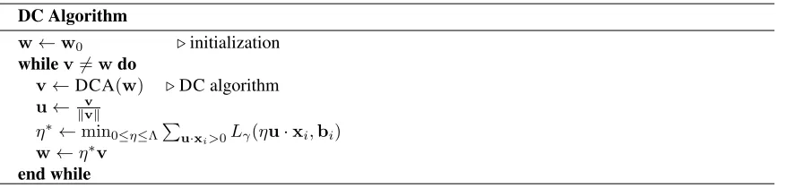
DC Algorithm

w_←w0 .initialization

whilev₆=wdo

v_←DCA(w) .DC algorithm u_←kv_vk

η∗_←min0≤η≤ΛPu·xi>0Lγ(ηu·xi,bi) w_←η∗v

end while

Figure 5: Pseudocode of our DC-programming algorithm.

The problem is equivalent to a QP (quadratic-programming). Indeed, by convex duality, there exists aλ >0

such that the above problem is equivalent to

min

w∈RNλkwk

2

+

m

X

i=1

si−δV(wt−1)·w

subject to(si≥ −w·xi)∧

h

si≥

1

γ w·xi−(1 +γ)b

(1)

i

i

which is a simple QP that can be tackled by one of many off-the-shelf QP solvers. Of course, the value ofλ

as a function ofΛdoes not admit a simple expression. Instead, we selectλthrough validation which is then equivalent to choosing the optimal value ofΛthrough validation.

We now address the problem of the DC algorithm converging to a local minimum. A common practice is to restart the DC algorithm at a new random point. Instead, we propose an algorithm that iterates along different local minima, with the guarantee of reducing the function at every change of local minimum. The algorithm is simple and is based on the observation that the functionLγis positive homogeneous. Indeed, for

anyη >0and(r,b),

Lγ(ηr, ηb) =−ηb(2)1ηr<ηb(2)−ηr1_ηb(2)_≤ηr≤ηb(1)+

ηr−(1 +γ)ηb(1)

γ 1ηb(1)_{<ηr<η(1+γ)b}(1)

=ηLγ(r,b).

Minimizing the objective function of (12) in a fixed directionu,kuk = 1, can be reformulated as follows:

min0≤η≤Λ Pm_i=1Lγ(ηu·xi,bi). Since foru·xi≤0the functionη7→Lγ(ηu·xi,bi)is constant and

equal to−b(2)_i , the problem is equivalent to solving

min

0≤η≤Λ

X

u·xi>0

Lγ(ηu·xi,bi).

Furthermore, sinceLγ is positive homogeneous, for alli ∈ [1, m]withu·xi > 0, Lγ(ηu·xi,bi) =

(u·xi)Lγ(η,bi/(u·xi)). Butη7→(u·xi)Lγ(η,bi/(u·xi))is av-function and thus the problem can

efficiently be optimized using the combinatorial algorithm for the no-feature case (Section5.1). This leads to the optimization algorithm described in Figure5. The last step of each iteration of our algorithm can be viewed as aline searchand this is in fact the step that reduces the objective function the most in practice. This is because we are then precisely minimizing the objective function even though this is for some fixed direction. Since in general this line search does not find a local minimum (we are likely to decrease the objective value in other directions that are not the one in which the line search was performed) running DCA helps us find a better direction for the next iteration of the line search.

6. Experiments

As mentioned before, a standard solution for solving this problem would be the use of a convex surrogate loss. In view of that, we compare against the solution of the regularized empirical risk minimization of the convex surrogate lossLαshown in Figure2(a) parametrized byα∈[0,1]and defined by

Lα(r,b) =

(

−r ifr < b(1)_+α(b(2)_−b(1)₎

(1−α)b(1)+αb(2) α(b(1)−b(2)₎

(r−b(1)) otherwise.

A second alternative consists of using ridge regression to estimate the first bid and of using its prediction as the reserve price. A third algorithm consists of minimizing the loss while ignoring the feature vectorsxi, i.e.,

solving the problemminr≤ΛPni=1L(r,bi). It is worth mentioning that this third approach is very similar to what advertisement exchanges currently use to suggest reserve prices to publishers. By using the empirical version of equation (2), we see that this algorithm is equivalent to finding the empirical distribution of bids and optimizing the expected revenue with respect to this empirical distribution as in (Ostrovsky and Schwarz, 2011) and (Cesa-Bianchi et al.,2013).

6.1 Artificial Data Sets

We generated4different synthetic data sets with different correlation levels between features and bids. For all our experiments, the feature vectorsx ∈ R21 were generated in as follows: ˜x ∈ R20 was sampled

from a standard Gaussian distribution andx = (˜x,1)was created by adding an offset feature. We now describe the bid generating process for each of the experiments as a function of the feature vectorx. For our first three experiments, shown in Figure6(a)-(c), the highest bid and second highest bid were set to

max

P21

i=1xi

+1,

P21

i=1

xi

2

+2

+ andmin

P21

i=1xi

+1,

P21

i=1

xi

2

+2

+ respectively, whereiis a Gaussian random variable with mean0. The standard deviation of the Gaussian noise was varied

over the set{0,0.25,0.5}.

For our last artificial experiment, we used a generative model motivated by previous empirical observa-tions (Ostrovsky and Schwarz,2011;Lahaie and Pennock,2007): bids were generated by sampling two values from alog-normal distribution with meansx·wandx·w

2 and standard deviation0.5, withwa random vector sampled from a standard Gaussian distribution.

For all our experiments, the parameters λ, γ and αwere selected respectively from the sets {2i_|

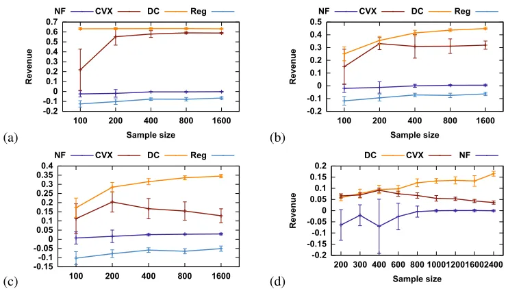
i ∈ [−5,5]},{0.1,0.01,0.001}, and{0.1,0.2, . . . ,0.9}via validation over a set consisting of the same number of examples as the training set. Our algorithm was initialized using the best solution of the convex surrogate optimization problem. The test set consisted of5,000examples drawn from the same distribution as the training set. Each experiment was repeated 10 times and the mean revenue of each algorithm is shown in Figure6. The plots are normalized in such a way that the revenue obtained by setting no reserve price is equal to0and the maximum possible revenue (which can be obtained by setting the reserve price equal to the highest bid) is equal to1. The performance of the ridge regression algorithm is not included in Figure6(d) as it was too inferior to be comparable with the performance of the other algorithms.

By inspecting the results in Figure6(a), we see that, even in the simplest noiseless scenario, our algorithm outperforms all other techniques. The reader could argue that these results are not surprising since the bids were generated by a locally linear function of the feature vectors, thereby ensuring the success of our algo-rithm. Nevertheless, one would expect this to be the case too for algorithms that leverage the use of features such as the convex surrogate and ridge regression. But one can see that this is in fact not true even for low levels of noise. It is also worth noticing that the use of ridge regression is actually worse than setting the reserve price to0. This fact can be easily understood by noticing that the square loss used in regression is symmetric. Therefore, we can expect several reserve prices to be above the highest bid, making the revenue of these auctions equal to zero. Another notable feature is that as the noise level increases, the performance of feature-based algorithms decreases. This is true for any learning algorithm: if the features are not relevant to the prediction task, the performance of the algorithm will suffer. However, for the convex surrogate algorithm, a more critical issue occurs: the performance of this algorithm actually decreases as the sample size increases, which shows that in general learning with a convex surrogate is not possible. This is an empirical verification of the inconsistency result provided in Section4.2. This lack of calibration can also be seen in Figure6(d), where in fact the performance of this algorithm approaches the use of no reserve price.

(a) -0.2 -0.1 0 0.1 0.2 0.3 0.4 0.5 0.6 0.7

100 200 400 800 1600

Rev

enue

Sample size

NF CVX DC Reg

(b) -0.2 -0.1 0 0.1 0.2 0.3 0.4 0.5

100 200 400 800 1600

Rev

enue

Sample size

NF CVX DC Reg

(c) -0.15-0.1 -0.05 0 0.05 0.1 0.15 0.2 0.25 0.3 0.35 0.4

100 200 400 800 1600

NF CVX DC Reg

(d) -0.2 -0.15 -0.1 -0.05 0 0.05 0.1 0.15 0.2

200 300 400 600 800 1000120016002400

Rev

enue

Sample size

DC CVX NF

Figure 6: Plots of expected revenue against sample size for different algorithms: DC algorithm (DC), convex surrogate (CVX), ridge regression (Reg) and the algorithm that uses no feature to set reserve prices (NF). For (a)-(c) bids are generated with different noise standard deviation (a) 0, (b) 0.25, (c) 0.5. The bids in (d) were generated using a generative model.

0 2 4 6 8 10

0

50

100

150

0

50

100

150

0 2 4 6 8 10

Reserve price

Frequenc

y

DC bid distribution

0 2 4 6 8 10

0

50

100

150

200

0

50

100

150

200

0 2 4 6 8 10

Reserve price

Frequenc

y

CVX bid distribution

0 2 4 6 8 10

0

200

400

600

800

0

200

400

600

800

0 2 4 6 8 10

Reserve price

Frequenc

y

Regression bid distribution

Figure 7: Distribution of reserve prices for each algorithm. The algorithms were trained on 800 samples using noisy bids with standard deviation0.5.

25 30 35 40 45 50 55

CVX NF DC HB NR

Rev

enue

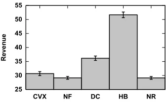
Figure 8: Results of the eBay data set. Comparison of our algorithm (DC) against a convex surrogate (CVX), using no features (NF), setting no reserve (NR) and setting reserve price to highest bid (HB).

6.2 Real-World Data Sets

Due to proprietary data and confidentiality reasons, we cannot present empirical results for AdExchange data. However, we were able to procure an eBay data set consisting of approximately 70,000 second-price auctions of collector sport cards. The full data set can be accessed using the following URL:http: //cims.nyu.edu/˜munoz/data. Some other sources of auction data are accessible (e.g., http: //modelingonlineauctions.com/datasets), but features are not available for those data sets. To the best of our knowledge, with the exception of the one used here, there is no publicly available data set for online auctions including features that could be readily used with our algorithm. The features used here include information about the seller such as positive feedback percent, seller rating and seller country; as well as information about the card such as whether the player is in the sport’s Hall of Fame. The final dimension of the feature vectors is78. The values of these features are both continuous and categorical. For our experiments we also included an extra offset feature.

Since the highest bid is not reported by eBay, our algorithm cannot be straightforwardly used on this data set. In order to generate highest bids, we calculated the mean price of each object (each card was generally sold more than once) and set the highest bid to be the maximum between this average and the second highest bid.

Figure8shows the revenue gained using different algorithms including our DC algorithm, using a con-vex surrogate, or the algorithm that ignores features. It also shows the results obtained by using no reserve price (NR) and the highest possible revenue obtained by setting the reserve price to the highest bid (HB). We randomly sampled2,000examples for training,2,000examples for validation and2,000examples for testing. This experiment was repeated10times. Figure8(b) shows the mean revenue for each algorithm and their standard deviations. The results of this experiment show that the use of features is crucial for revenue optimization. Indeed, setting an optimal reserve price for all objects seems to achieve the same revenue as no reserve price. Instead, our algorithm achieves a 22% increase on the revenue obtained by not setting a reserve price whereas the non-calibrated convex surrogate algorithm only obtains a 3% revenue improvement. Furthermore, our algorithm is able to obtain as much as 70% of the achievable revenue with knowledge of the highest bid.

7. Conclusion

Acknowledgments

Appendix A. Contraction Lemma

The following is a version of Talagrand’s contraction lemmaLedoux and Talagrand(2011). Since our defini-tion of Rademacher complexity does not use absolute values, we give an explicit proof below.

Lemma 14 LetH be a hypothesis set of functions mappingX toRandΨ1, . . . ,Ψm,µ-Lipschitz functions for some

µ >0. Then, for any sampleSofmpointsx1, . . . , xm∈ X, the following inequality holds

1 mEσ

" sup

h∈H m

X

i=1

σi(Ψi◦h)(xi)

# ≤ µ

mEσ

" sup

h∈H m

X

i=1

σih(xi)

#

=µRbS(H).

Proof The proof is similar to the case where the functionsΨiare all equal. Fix a sampleS= (x1, . . . , xm).

Then, we can rewrite the empirical Rademacher complexity as follows:

1 mEσ

h sup

h∈H m

X

i=1

σi(Ψi◦h)(xi)

i = 1

mσ1,...,σEm−1

h E

σm h

sup

h∈H

um−1(h) +σm(Ψm◦h)(xm)

ii

,

whereum−1(h) =Pm_i=1−1σi(Ψi◦h)(xi). Assume that the suprema can be attained and leth1, h2 ∈Hbe the hypotheses satisfying

um−1(h1) + Ψm(h1(xm)) = sup h∈H

um−1(h) + Ψm(h(xm))

um−1(h2)−Ψm(h2(xm)) = sup h∈H

um−1(h)−Ψm(h(xm)).

When the suprema are not reached, a similar argument to what follows can be given by considering instead hypotheses that are-close to the suprema for any >0.

By definition of expectation, sinceσmuniform distributed over{−1,+1}, we can write

E

σm h

sup

h∈H

um−1(h) +σm(Ψm◦h)(xm)

i = 1

2hsup∈H

um−1(h) + (Ψm◦h)(xm) +

1 2hsup∈H

um−1(h)−(Ψm◦h)(xm)

= 1

2[um−1(h1) + (Ψm◦h1)(xm)] + 1

2[um−1(h2)−(Ψm◦h2)(xm)].

Lets= sgn(h1(xm)−h2(xm)). Then, the previous equality implies

E

σm h

sup

h∈H

um−1(h) +σm(Ψm◦h)(xm)

i ≤ 1

2[um−1(h1) +um−1(h2) +sµ(h1(xm)−h2(xm))]

= 1

2[um−1(h1) +sµh1(xm)] + 1

2[um−1(h2)−sµh2(xm)]

≤ 1 2hsup∈H

[um−1(h) +sµh(xm)] +

1 2hsup∈H

[um−1(h)−sµh(xm)]

= E

σm h

sup

h∈H

um−1(h) +σmµh(xm)

i

,

where we used theµ−Lipschitzness ofΨmin the first equality and the definition of expectation overσmfor

the last equality. Proceeding in the same way for all otherσi’s (i6=m) proves the lemma.

Appendix B. Proof of Theorem

7

Proof We first show that the functionsLnare uniformly bounded for anyb:

|Ln(r, b)|=

Z r

0

L0n(r, b)dr

≤ Z M 0 max L 0

n(0, b)

, L 0

n(M, b)

dr ≤ Z M 0

where the first inequality holds since, by convexity, the derivative ofLn with respect toris an increasing

function.

Next, we show that the sequence(Ln)n∈N is also equicontinuous. It will follow then by the theorem of Arzela-Ascoli that the sequenceLn(·, b)converges uniformly toLc(·, b). Letr1, r2 ∈ [0, M], for any

b∈[0, M]we have

|Ln(r1, b)−Ln(r2, b)| ≤ sup

r∈[0,M]

L

0

n(r, b)

|r1−r2|

= max L

0

n(0, b)

,

L

0

n(M, b))

|r1−r2|

≤K|r1−r2|,

where, again, the convexity ofLnwas used for the first equality. LetFn(r) =Eb∼D[Ln(r, b)]andF(r) =

Eb∼D[Lc(r, b)]. Fnis a convex function as the expectation of a convex function. By the theorem of

Arzela-Ascoli, the sequence(Fn)n admits a uniformly convergent subsequence. Furthermore, by the dominated

convergence theorem, we have(Fn(r))nconverges pointwise toF(r). Therefore, the uniform limit ofFn

must beF. This implies that

min

r∈[0,M]F(r) =n→lim+∞r∈min[0,M]Fn(r) =n→lim+∞Fn(rn) =F(r ∗

),

where the first and third equalities follow from the uniform convergence ofFntoF. The last equation implies

thatLcis consistent withLe. Furthermore, the functionLc(·, b)is convex since it is the uniform limit of convex

functions. It then follows by Proposition6thatLc(·, b)≡Lc(0, b) = 0.

Appendix C. Consistency of

L

Lemma 15 LetHbe a closed, convex subset of a linear space of functions containing 0 and leth∗γ= argminh∈HLγ(h).

Then, the following inequality holds: E x,b

h

h∗γ(x)1I2(x,b)

i ≥ 1

γxE,b h

h∗γ(x)1I3(x,b)

i

.

Proof Let0< λ <1. SinceH is a convex set, it follows thatλh∗γ ∈H. Furthermore, by the definition of

h∗γ, we must have:

E x,b

h

Lγ(h

∗

γ(x),b)

i ≤ E

x,b h

Lγ(λh

∗

γ(x),b)

i

. (14)

Ifh∗γ(x) < 0, thenLγ(h∗γ(x),b) = Lγ(λh∗γ(x)) = −b(2) by definition ofLγ. If on the other hand

h∗γ(x)>0, sinceλh

∗

γ(x)< h

∗

γ(x), we must have that for(x,b)∈I1 Lγ(hγ∗(x),b) =Lγ(λh∗γ(x),b) =

−b(2)too. Moreover, from the fact thatLγ ≤ 0andLγ(h∗γ(x),b) = 0for(x,b) ∈ I4 it follows that

Lγ(h∗γ(x),b)≥Lγ(λh∗γ(x),b)for(x,b)∈I4, and therefore the following inequality trivially holds:

E x,b

h

Lγ(h∗γ(x),b)(1I1(x,b) +1I4(x,b))

i ≥ E

x,b h

Lγ(λh∗γ(x),b)(1I1(x,b) +1I4(x,b))

i

. (15)

Subtracting (15) from (14) we obtain

E x,b

h

Lγ(h

∗

γ(x),b)(1I2(x,b) +1I3(x,b))

i ≤ E

x,b h

Lγ(λh

∗

γ(x),b)(1I2(x,b) +1I3(x,b))

i

.

Rearranging terms shows that this inequality is equivalent to

E x,b

h (Lγ(λh

∗

γ(x),b)−Lγ(h

∗

γ(x),b))1I2(x,b)

i ≥ E

x,b h

(Lγ(h

∗

γ(x),b)−Lγ(λh

∗

γ(x),b))1I3(x,b)

i

(16)

Notice that if(x,b) ∈ I2, thenLγ(h∗γ(x),b) = −h

∗

γ(x). Ifλh

∗

γ(x) > b(2)too thenLγ(λh∗γ(x),b) =

−λh∗γ(x). On the other hand ifλh

∗

γ(x)≤b(2)thenLγ(λh∗γ(x),b) =−b(2)≤ −λh

∗

γ(x). Thus

E(Lγ(λh∗γ(x),b)−Lγ(h∗γ(x),b))1I2(x,b))≤(1−λ)E(h

∗

1. λh∗γ(x)≤b(1);

2. λh∗γ(x)> b(1).

In the first case, we know thatLγ(h∗γ(x),b) = _γ1(h∗γ(x)−(1 +γ)b(1))>−b(1)(sinceh∗γ(x)> b(1)for

(x,b)∈I3). Furthermore, ifλh∗γ(x)≤b(1), then, by definitionLγ(λh∗γ(x),b) = min(−b(2),−λh

∗

γ(x))≤

−λh∗γ(x). Thus, we must have:

Lγ(h

∗

γ(x),b)−Lγ(λh

∗

γ(x),b)> λh

∗

γ(x)−b

(1)

>(λ−1)b(1)≥(λ−1)M, (18)

where we used the fact thath∗γ(x)> b(1)for the second inequality and the last inequality holds sinceλ−1<

0.

We analyze the second case now. Ifλh∗γ(x) > b(1), then for(x,b) ∈ I3 we have Lγ(h∗γ(x),b)−

Lγ(λh∗γ(x),b) = 1γ(1−λ)h

∗

γ(x). Thus, letting∆(x,b) =Lγ(h∗γ(x),b)−Lγ(λh∗γ(x),b), we can lower

bound the right-hand side of (16) as:

E x,b

h

∆(x,b)1I3(x,b)

i = E

x,b h

∆(x,b)1I3(x,b)1{λh∗

γ(x)>b(1)} i

+ E x,b

h

∆(x,b)1I3(x,b)1{λh∗

γ(x)≤b(1)} i

≥ 1−λ γ xE,b

h

h∗γ(x)1I3(x,b)1{λh∗

γ(x)>b(1)} i

+ (λ−1)MP h

h∗γ(x)> b(1)≥λh

∗

γ(x)

i

,

(19)

where we have used (18) to bound the second summand. Combining inequalities (16), (17) and (19) and dividing by(1−λ)we obtain the bound

E x,b

h

h∗γ(x)1I2(x,b)

i ≥ 1

γxE,b h

h∗γ(x)1I3(x,b)1{λh∗

γ(x)>b(1)} i

−MP h

h∗γ(x)> b

(1)

≥λh∗γ(x)

i

.

Finally, taking the limitλ→1, we obtain

E x,b

h

h∗γ(x)1I2(x,b)

i ≥ 1

γxE,b h

h∗γ(x)1I3(x,b)

i

.

Taking the limit inside the expectation is justified by the bounded convergence theorem andP[h∗γ(x)> b(1)≥

λh∗γ(x)]→0holds by the continuity of probability measures.

Proposition 16 For anyδ >0, with probability at least1−δover the choice of a sampleSof sizem, the following holds for allγ∈(0,1]andh∈H:

Lγ(h)≤Lbγ(h) +

2

γRm(H) +M

"s

log log₂ 1

γ m + s log1 δ 2m # .

Proof Consider two sequences(γk)k≥1and(k)k≥1, withk∈(0,1). By Theorem9, for any fixedk≥1,

P

Lγk(h)−Lbγk(h)> 2 γk

Rm(H) +M k

≤exp(−2m2k).

Choosek=+

q

logk

m , then, by the union bound,

P

∃k:Lγk(h)−Lbγk(h)> 1 γk

Rm(H) +M k

≤X

k≥1

exp

−2m(+p(logk)/m)2

≤ X

k≥1

1/k2

exp(−2m2)

=π

2

6 exp(−2m

2