Incremental Identification of Qualitative Models of Biological Systems
using Inductive Logic Programming
Ashwin Srinivasan∗ [email protected]
IBM India Research Laboratory
4-C, Institutional Area, Vasant Kunj Phase II New Delhi 110 070, India
Ross D. King [email protected]
Department of Computer Science University of Wales, Aberystwyth Ceredigion, Wales, UK
Editor: Stefan Wrobel
Abstract
The use of computational models is increasingly expected to play an important role in predict-ing the behaviour of biological systems. Models are bepredict-ing sought at different scales of biological organisation namely: sub-cellular, cellular, tissue, organ, organism and ecosystem; with a view of identifying how different components are connected together, how they are controlled and how they behave when functioning as a system. Except for very simple biological processes, system iden-tification from first principles can be extremely difficult. This has brought into focus automated techniques for constructing models using data of system behaviour. Such techniques face three principal issues: (1) The model representation language must be rich enough to capture system be-haviour; (2) The system identification technique must be powerful enough to identify substantially complex models; and (3) There may not be sufficient data to obtain both the model’s structure and precise estimates of all of its parameters. In this paper, we address these issues in the following ways: (1) Models are represented in an expressive subset of first-order logic. Specifically, they are expressed as logic programs; (2) System identification is done using techniques developed in Inductive Logic Programming (ILP). This allows the identification of first-order logic models from data. Specifically, we employ an incremental approach in which increasingly complex models are constructed from simpler ones using snapshots of system behaviour; and (3) We restrict ourselves to “qualitative” models. These are non-parametric: thus, usually less data are required than for identifying parametric quantitative models. A further advantage is that the data need not be pre-cise numerical observations (instead, they are abstractions like positive, negative, zero, increasing, decreasing and so on). We describe incremental construction of qualitative models using a simple physical system and demonstrate its application to identification of models at four scales of bio-logical organisation, namely: (a) a predator-prey model at the ecosystem level; (b) a model for the human lung at the organ level; (c) a model for regulation of glucose by insulin in the human body at the extra-cellular level; and (d) a model for the glycolysis metabolic pathway at the cellular level.
Keywords: ILP, qualitative system identification, biology
1. Introduction
There is a general move in biology from seeking an understanding at the level of individual units (genes, proteins and so on) to an understanding at the system-level. Identifying single genes, pro-teins or metabolite levels cannot be expected to yield an answer to systemic behaviour any more than a list of radio parts could explain its behaviour (a point made in Lazebnik’s humourous and perceptive article: Lazebnik, 2002). What is needed is an understanding of the function of each part and, crucially, how these components are connected, how they are controlled and the dynamic behaviour of the system as a whole. Biology, which for the last decade or so has been pre-occupied with establishing the “parts-list” is now moving to address these other issues. Besides the obvious scientific value of understanding whole systems, substantial benefits are expected to follow in clin-ical medicine. This is concerned with the application of computation and applied mathematics to improve existing pharmaceutical and medical practices. It is expected that results in systems-level biology will allow a better understanding of the nature of diseases, leading to a targeted design of new drugs and drug treatments. The importance of adopting a systemic approach to biology is not new: there are statements in Darwin’s Origin that clearly anticipate this need. Its relevance in the modern biological context is summarised in a recent article in Science (W.Bialek and D.Botstein, 2004):
The basic nature and goals of biological research is changing fundamentally. In the past, biological processes and the underlying genes, proteins, other molecules, and en-vironmental factors were of necessity studied one by one in relative isolation. In con-trast, today we are no longer satisfied with studies or answers that place each of these in a larger context. We now know that there are tens of thousands of genes encoded in the genome and that simple perturbations such as . . . heat shock, alter the expression of thousands of them . . . New goals are in sight, namely robust mathematical models and computer simulations that faithfully predict the behaviour of entire biological systems.
Some substantial research effort is being expended in trying to achieve these goals. The Physiome Project for example (seehttp://www.physiome.org/) lists its principal aim as being “to under-stand and describe the human organism, its physiology and pathophysiology quantitatively.” This it hopes to achieve by using models at different levels (molecular to organ) that “include everything from diagrammatic schema suggesting relationships to fully quantitative computational models.” Similarly, the United Kingdom’s main research funding body in biology (the BBSRC) has invested over 15 million pounds in centres for integative systems biology: “the aim is to support research in such a way that all the components of the system under study can be researched at all relevant levels of biological organisation. It necessitates being able to to handle large experimental data sets and having the expertise and capacity to manipulate these and combine them with the theoretical base to develop new predictive and holistic models of how living systems function.” (see Bioscience for
So-ciety: A Ten Year Vision, January 2003 at
http://www.bbsrc.ac.uk/about/plans reports/vision.html).
proceed from first principles (for example, balance equations, energy conservation and so on), the complexity of biological systems often force a much more experimental approach. The modeller selects those physical processes believed to be important, constructs a model and checks if solu-tions match the observed data. If not, the procedure is repeated until an adequate model is found. For example, a first attempt at modelling oxygen transport to red blood cells may consider a model that accounted for convection, diffusion and chemical reaction (these are the principal physical pro-cesses involved). In fact, convection makes a negligible contribution and reaction is only important for sick lungs. Once it is known that only the diffusion term is important, a parametric equation can be found relatively easily.
Broadly speaking, system identification can be viewed as “the field of modelling dynamic sys-tems from experimental data” (Soderstrom and Stoica, 1989). We can distinguish here between: (a) classical system identification techniques, developed by control engineers and econometricians; and (b) machine learning techniques for system identification, developed by computer scientists. While the kinds of models identified by the two kinds of techniques are different, neither provides a foolproof method that can be employed without user interaction.
Classical system identification has concentrated on models largely constrained to be either ordi-nary differential equations (ODEs) or linear difference equations of some order. With this constraint on model structure, the input-output behaviour of the system is observed over a time interval and some statistical method is used to estimate parameters in the model. In its most general formula-tion, system identification proceeds by repeated estimation of both structure and parameters until an acceptable model is found. In practice, a small set of structures are given a priori and the proce-dure reduces to one of parameter estimation. Classical techniques have been used to identify linear time-invariant models for purposes of extracting control strategies (in engineering) or time-series predictions (in economics).
In this paper we are concerned instead with using machine learning techniques for system iden-tification. Specifically, our interest is in methods that: (a) are not restricted to specific model struc-tures; and (b) allow the incorporation of domain knowledge both to specify constraints on acceptable model structures and to direct the search through the space of acceptable structures. We believe both these features to be necessary in any empirical approach for identifying biological systems from data. Of the machine learning methods available that are capable of satisfying these requirements, those developed under the framework of Inductive Logic Programming (ILP) are amongst the most powerful. There are two reasons for this. First, the rich logic-based formalism used by ILP methods allows them to represent and identify a wide variety of relational descriptions. Second, ILP meth-ods are unusual in that they make explicit provisions for the incorporation of domain knowledge to guide the model identification process. This includes mechanisms for the requirement in (b) above. One question that is often raised in the context of ILP is that of efficiency. In the context here, this translates to asking if ILP methods are efficient enough to identify significantly complex biological models? As long as it is reasonable to identify such models in an incremental manner, we believe the answer to this question is “yes” and demonstrate this with the identification of four fairly complex systems at different scales of biological organisation (a predator-prey model at the ecosystem level; a model for the human lung at the organ level; a model for glucose regulation at the extra-cellular level; and the glycolysis metabolic pathway at the cellular level).
data. While substantial amounts of quantitative data are being generated at some lower levels of biological organisation (a prominent example is provided by the use of DNA microarray data to es-timate mRNA levels in a cell), quality is still variable: it is possible, for example to get very different expression profiles for the same tissue using different microarray technologies (Kuo et al., 2002). At higher levels (for example, at the organ or ecosystem level), data are sparse, although of perhaps better quality. In all cases, we believe it to be substantially easier and more reliable to obtain data that are of a qualitative nature. For example, it may be relatively easier to decide whether certain metabolites are present or absent in a cell, whether their levels have been increasing or decreasing and so on, rather than obtain precise measurements of the metabolites. In this paper, we will be concerned exclusively with system identification from such qualitative data. The resulting models are non-parametric: that is, parameter estimation is not required and data are only needed to identify the model structure. Clearly, these qualitative models cannot be treated as being equivalent to their quantitative counterparts. Nevertheless, they can be used to simulate possible system behaviours and may be much more understandable to a non-mathematical biologist than a quantitative model like a differential equation.
The rest of the paper is organised as follows. Section 2 describes an established approach to qualitative reasoning about dynamic systems. This involves the use of qualitative constraints which form the building blocks of qualitative models (these models include abstractions of ordinary dif-ferential equations). Section 3 describes informally the the basics of an ILP system used to identify qualitative models. This includes a variant that performs an incremental identification of increas-ingly complex models. Section 5.1 demonstrates this form of identification using a model physical system. The application to biological systems is in Section 6. Section 7 examines the automatic identification of stages for the incremental learner. Section 8 concludes the paper. Appendix A provides details of the ILP system used for incremental system identification. Appendix B provides details of the procedure for multi-stage decomposition.
2. Constraint-Based Qualitative Reasoning
Figure 1 (slightly modified from Bratko, 2001) shows four different qualitative abstractions of some numerical statements: (a) numbers are represented by intervals (marked by some distinguished values like zero,end, inf and so on); (b) derivatives are represented by directions of change (like
inc); (c) functions are represented by monotonic relations (like MPLUS denoting “monotonically
increasing”); and (d) entire sequences of behaviour are represented by qualitative statements that specify a qualitative values and directions of change.
Reasoning with qualitative abstractions requires a calculus: we propose to use the constraint-based formulation used in the qualitative simulation program QSIM (Kuipers, 1994) (here we pro-vide an informal description along the lines described by Bratko 2001). In this, variables take qualitative values from domains. Domains are defined by a name and some ordered set of distin-guished values called landmarks. For example, the variable Amount in Fig. 1 could be from the domain level with landmarks min f,0,in f . A qualitative state of a variable is usually denoted by
Domain : QVal where QVal is represented as ahQmag,Qdiripair, sometimes written Qmag/Qdir.
Qdir is the qualitative rate of change of the variable, which has a fixed, three-valued resolution (the
Quantitative Statement Qualitative Statement (a) Level(3.2 s) =2.6 cm Level(t1) =zero...in f
(b) dtdLevel(3.2 s) =0.12 m/s DERIV(Level(t1)) =std
(c) Amount=Level×Level MPLUS(Level,Amount)
(d) Time Amount
0.0 0.00 Amount(zero...end) =
0.1 0.02 zero...in f/inc
. . . . . . . .
159.3 62.53
Figure 1: Qualitative abstractions of numerical data (from Bratko, 2001).
The qualitative state of a system is simply a list of the qualitative states of the system’s variables and a qualitative behaviour is a list of consecutive qualitative states.
Reasoning is accomplished using constraints. In this approach, pioneered by Kuipers (1994), there are four principal constraints:ADD(A,B,C), for addition of qualitative variablesAandBto give
C;1MULT(A,B,C), to denoteA×B=C;MINUS(A,B), for sign inversionA=−B; andDERIV(A,B), to denote thatBis the a derivative ofA. In this paper, we will also useSUB(A,B,C)to denoteA −
B =C. In addition to these, two functional constraints are also used: MPLUS(A,B), to denote that whenAincreases thenBincreases as well; andMMINUS(A,B), to denote that whenAincreases then
Bdecreases. We will henceforth refer to these constraints as “the QSIM constraints”.
Figure 2 shows a qualitative model for a simple physical system, expressed in terms of the QSIM constraints. A qualitative behaviour of this system—that is, a sequence of qualitative states of the system variablesLa,LbandFabthat satisfy the model’s constraints—is shown in Fig. 3
A number of advantages have been proposed for using qualitative models. First, in some cases they may be more appropriate than quantitative models. This is particularly so if quantitative mea-surements are either difficult to obtain or are noisy and what is of interest are the essential properties of the system. Second, the models are quite comprehensible. Both these features are particularly relevant to the modelling of biological systems. There is an additional advantage for automatic system identification of the kind we propose here. Since qualitative models are non-parametric all computational effort is focussed on identifying the model structure. This typically requires data of both less precision and quantity than that required for identification of quantitative models.
1. Constraints apply to the qualitative states ofA,BandC. Recall that these are of the form Domain : Qmag/Qdir. Thus, theADDconstraint ensures that both magnitudes and directions of change are consistent. ThusADD(level : 0/inc,level : 0...in f/std,level : in f/inc)is true, butADD(level : 0...in f/inc,level : in f/std,level : 0...in f/inc)is not (0...in f+in f 6=0...in f ). Similarly,ADD(level : 0...in f/inc,level : 0...in f/std,level : 0...in f/inc)is true, but
ADD(level : 0...in f/inc,level : 0...in f/std,level : 0...in f/std)is not (inc+std6=std). It should also be apparent, that while quantitative addition is functional (the sum of a pair of numbers is a unique number) , qualitative addition ones is relational (that is, for a pair of qualitative states forAandB,ADDmay be true for more than one qualitative state for
d dt
d dt
La
Lb
Fab
B A
Diagrammatic Model:
+
La
Fab Fba
Lb Diff
M+
Qualitative Model:
DERIV(La,Fba) DERIV(Lb,Fab) ADD(Lb,Diff,La) MPLUS(Diff,Fab) MINUS(Fab,Fba)
Figure 2: The U-tube and its qualitative model. There are three (measurable) system variables: the water-level in arm A (La); the water-level in arm B (Lb); and the flow of water from A to B (Fab). The diagrammatic model shows the system components involved (two differentiators, an adder, an inverter, and a monotonic function generator) and their inter-connections. The qualitative model expresses the same information as a conjunction of constraints (here, we have used the QSIM constraints described in the paper).
La Lb Fab
level : 0/std level : 0/std f low : 0/std level : 0/inc level : 0...in f/dec f low : min f...0/inc level : 0...in f/dec level : 0/inc f low : 0...in f/dec level : 0...in f/dec level : 0...in f/inc f low : 0...in f/dec level : 0...in f/std level : 0...in f/std f low : 0/std level : 0...in f/inc level : 0...in f/dec f low : min f...0/inc
Figure 3: A qualitative behaviour of the U-tube that is consistent with the qualitative model in Fig. 2. The rows are example states of the qualitative variables and have no implied ordering.
3. Model Identification using Inductive Logic Programming
directed acyclic graph representation of possible models. In this representation, a pair of models are connected in the graph if one can be transformed into another by an operation called “refinement”. Figure 4 shows some parts of a graph for the U-tube in which a model is refined to another by the addition of a qualitative constraint. An optimal search procedure (branch-and-bound, for example) traverses this graph in some order, at all times keeping the cost of the best nodes so far. Whenever a node is reached where it is certain that it and all its descendents have a cost higher than that of the best nodes, then the node and its descendents are removed from the search. A portion of the search tree commencing at /0for one such search is shown in Fig. 5.
DERIV(La,Fab) DERIV(Lb,Fba) DERIV(La,Fab) ADD(Lb,Diff,La) ADD(Lb,Diff,La) DERIV(La,Fab) DERIV(Lb,Fba) DERIV(La,Fab) DERIV(Lb,Fba) ADD(Lb,Diff,La) MPLUS(Diff,Fab) MPLUS(Diff,Fab) DERIV(La,Fab) ADD(Lb,Diff,La) DERIV(La,Fab) DERIV(Lb,Fba) MINUS(Fab,Fba) ADD(Lb,Diff,La) DERIV(La,Fab) DERIV(Lb,Fba) MINUS(Fab,Fba) MPLUS(Diff,Fab) DERIV(La,Fab) DERIV(Lb,Fba) MINUS(Fab,Fba) MPLUS(Diff,Fab) DERIV(La,Fab) DERIV(Lb,Fba) ADD(Lb,Diff,La) MINUS(Fab,Fba) Φ ADD(Lb,Diff,La) DERIV(Lb,Fba) MPLUS(Diff,Fab) DERIV(La,Fab) MPLUS(Diff,Fab) ADD(Lb,Diff,La) MINUS(Fab,Fba) ADD(Lb,Diff,La) ... ... ... ... ... ... ... ... ... ... ... ... ... ... ... ... ...
DERIV(La,Fab) MINUS(Fab,Fba) ADD(Diff,Lb,La)
DERIV(Lb,Fba)
Figure 4: Portions of a refinement graph of models for the U-tube.
Enumerative procedures like branch-and-bound works best if the cost function is monotonic. That is, the score of each node in the search tree is at least as bad as all its descendents (this allows the nodes and its descendents to be removed from the search). The procedure is optimal in the sense that it is guaranteed to find the best solution(s). However in the worst case, it may require examining the entire search space.
ADD(Lb,Diff,La)
DERIV(Lb,Fba) MINUS(Fab,Fba)
DERIV(La,Fab) MPLUS(Diff,Fab)
MPLUS(Diff,Fab) DERIV(Lb,Fba)
MPLUS(Diff,Fab) ADD(Lb,Diff,La)
MINUS(Fab,Fba) MPLUS(Diff,Fab) DERIV(La,Fab)
MPLUS(Diff,Fab)
MPLUS(Diff,Fab) DERIV(La,Fab) DERIV(Lb,Fba)
MPLUS(Diff,Fab) DERIV(La,Fab) ADD(Lb,Diff,La)
MPLUS(Diff,Fab) DERIV(La,Fab) MINUS(Fab,Fba)
MPLUS(Diff,Fab) DERIV(La,Fab) DERIV(Lb,Fba) ADD(Lb,Diff,La)
MPLUS(Diff,Fab) DERIV(La,Fab) DERIV(Lb,Fba) MINUS(Fab,Fba)
ADD(Lb,Diff,La) MINUS(Fab,Fba) DERIV(Lb,Fba) DERIV(La,Fab) MPLUS(Diff,Fab)
Φ
Figure 5: Portions of the search tree explored when searching for models for the U-tube. The search starts from /0.
1. Background knowledge B. These are statements, usually written in some formal language that specify domain-specific information. We will include in this domain-specific constraints on the kinds of models that are acceptable (or unacceptable, if easier); and directions to the search procedure that allow the system to avoid useless search paths. Examples of these for qualitative model identification are:
(a) Definitions for qualitative constraints like DERIV, MPLUS, ADD and so on, along with appropriate dimensionality checks etc. to ensure their correct usage.
(b) A constraint specifying that models must not contain relations that are redundant. For example, the relation ADD(Diff,Lb,La) is redundant if the model already has
constraints. This prevents relations likeADD(Lb,Fab,La)from appearing in the model (Fabbeing a flow has different units of measurement to the levelLb).
(c) A directive that the search need not examine models that explain below some proportion of the observed behaviours (more on “explain” in a moment).
2. Examples E. These are the observed data. For qualitative model identification, these would be qualitative observations of system behaviour of the form shown in Fig. 3. ILP systems also accept counter-examples of system behaviour. Since this is difficult to obtain for the problems we are concerned with, we do not pursue this further here. Given a set of examples,
H is said to explain an observation e if H is consistent with B and e logically follows from B
and H (see Appendix A for a precise mathematical formulation). For example, given correct definitions for the qualitative constraintsDERIV,MPLUS,ADDandMINUSas background knowl-edge, the qualitative model described by the conjunctionDERIV(La,Fab)∧DERIV(Lb,Fba)
∧ADD(Lb,Diff,La)∧MPLUS(Diff,Fab)∧MINUS(Fab,Fba)is an explanation of the ex-amples in Fig. 3.
3. Refinement operator ρ. This function defines the set of descendents for each node in the
refinement graph. With most ILP systems, the set of descendents of a node are (minimal) generalisations or specialisations of the node. Roughly speaking, for qualitative models, gen-eralisations correspond either: to removing one or more qualitative components from the dia-grammatic model; or to “disconnecting” qualitative components from each other. Conversely, specialisations correspond to adding new components or connecting existing components.
4. Cost function f . This is a real-valued function for each node in the refinement graph. As mentioned earlier, monotonic cost functions are of some importance. A simple cost function satisfying this property in Fig. 4 is f(H) =−P, where P is the number of examples explained
by model H. If every element H0ofρ(H)contains at least one additional constraint, it can be shown that number of examples explained by H0 (and recursively, all its descendents) would be at most P. It follows therefore that the cost of H is no worse than any of its descendents. In practice such a cost function is too simple to be of use (the search would trivially return the most general model), and modifications are made either to: (a) incorporate a trade-off between the explanatory power of the model and its complexity (Muggleton, 1996); or (b) include additional constraints in the background knowledge that prevent the selection of trivial models.
A description of an ILP implementation that uses these components can be found in Section A.2.
4. Identification of Qualitative Models
Model-identification systems that allowed intermediate variables were developed independently by Richards et al. (1992) and Bratko et al. (1992). Both use general-purpose ILP learners (although in different ways) and the principal advantages and shortcomings of these approaches and a later program called QSI (Say and Kuru, 1996) have been documented elsewhere (Coghill et al., 2005).
More recently, the QOPH system for identifying qualitative models exploited the possibility of providing the ILP system ALEPH with a special-purpose refinement operator (Coghill et al., 2002). This operator, with certain “built-in” constraints on acceptable qualitative models, is used by ALEPH to search the space of possible models. Extensive experiments are reported by Coghill et al. (2002) on the reconstruction of some model physical systems. While the results are promising, the scalability of the approach is unclear, since: (a) Model identification is assumed to be possible in a single step. Some simple complexity arguments (see Section A.2) suggest that the complexity of this task grows exponentially with the number of constraints in the model (this is the primary motivation for the incremental approach described in the next section); and (b) The special-purpose refinement operator is difficult to modify and its properties are difficult to analyse. Although not using a general-purpose ILP system, Suc and colleagues have proposed a hybrid approach of com-bining a logic-based qualitative learner followed by numeric modelling to construct quantitative models of systems (Suc et al., 2003). The approach, called Q2-learning, first constructs “qualitative model trees”. These are like decision trees, with monotonic QSIM constraints in the leaves. These constraints are then used to direct the construction of quantitative models (usually linear models). The success of this approach depends on the availability and quality of numeric data and the sys-tem being modelled by a composition of quantitative models (for example, like piecewise linear models).
The advantages of using of a purely qualitative representation for modelling metabolic pathways has been recently advocated (King et al., 2005). In that paper, a special-purpose system is used to generate possible models for the glycolysis pathway. The approach we propose here differs from that in two principal ways. First, it is a general approach as opposed to a specialised one for metabolic pathways. Second, the complexity of the implementation by King and his co-workers is of the same order as QOPH implementation. The incremental approach described in the next section will usually be significantly more efficient.
5. Incremental Model Identification with ILP
Modern ILP systems are largely “one-shot” model constructors. That is, given B,E,ρand f , they attempt to identify models with the lowest cost in a single search. While this approach has been rea-sonably successful in the identification of small to medium-sized models (for example, qualitative models containing no more than 4 to 5 constraints), it is unclear whether the approach can scale up to the identification of substantially complex models. For example, the worst-case bound in Remark 2 in Section A.2 grows exponentially in the number of qualitative constraints in the model.
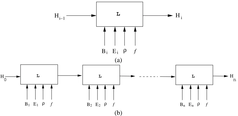
previous stage. Formally the incremental learner is principally provided with: (a) an initial set of models H0; (b) a sequence of pairs(Bi,Ei)corresponding to the background knowledge and exam-ples for each stage i (the Biand Eido not all have to be different); (c) a general-purpose refinement
operatorρfor all stages; and (d) a cost function f for all stages. The task of the incremental learner is to construct a set of models from this data (see Fig. 6 and Appendix A).
Hi−1 Hi
Bi Ei
L
ρ f (a)
B2 E2 ρ f
L
B1 E1 ρ f
L
Bn En ρ f
L
H H
0 n
(b)
Figure 6: Incremental model identification with ILP. The basic element shown in (a) consists of an ILP learnerL that takes as input a set of models, background knowledge, examples, a refinement operatorρand a cost function f . In (b), this basic unit is repeatedly used to construct a model in n stages. “One-shot” model identification by normal ILP systems is a special case of this process, with n=1 and H0={/0}(here /0denotes the empty model).
The actual implementation in Section A.2 contains some additional aspects which are not shown in Fig. 6 (and similar figures in Section 6) for simplicity:
1. A refinement operator that performs both generalisations and specialisations can completely revise models found at a previous stage. However, this is computationally expensive. In-stead, we use a refinement operator ρA that is restricted to performing specialisations only
(for qualitative models, this amounts to adding qualitative constraints and connecting exist-ing qualitative components). To correct partially for this shortcomexist-ing, models are subject to a limited generalisation before submission to any L. For qualitative models, this translates to retaining the qualitative components found at the previous stage but disconnecting some or all components, respecting any constraints provided on the usage of the components (in ILP terminology, this amounts to removing variable co-references, respecting any language constraints provided). This allows the incremental procedure to perform a particular kind of revision of models found at the previous stage;
3. A cost function fBayesdescribed in Muggleton (1996) is used. For qualitative models, this
per-forms a trade-off between the likelihood of a qualitative model and its complexity (a quantity related to the number of constraints in the model); and
4. An upper-bound is provided on the amount of search to be conducted by anyL.
Bi Ei
Hi−1 L Hi
ρ f
G S
A Bayes
Figure 7: A more accurate representation of the implementation of the basic element used in this paper. HereGperforms a limited generalisation of the input models, and can be eliminated for refinement operators that perform both generalisations and specialisations.Sperforms a random selection of the output models and can be eliminated if all models produced by
L are sent to the next stage. ρA is a refinement operator that performs specialisations
only; and fBayesis a Bayesian cost function. For simplicity, we will not showGandSin
subsequent figures.
A more accurate representation of the basic element of the incremental learner, as implemented by the procedures in Section A.2, is shown in Fig. 7. With these implementation choices it can be shown that, for identification of qualitative models, the size of the search space of such an in-cremental procedure is dominated by maximum number of additional qualitative constraints that need to be identified at any one of the stages (see Section A.2 for the details). The savings over a non-incremental approach can be substantial, but two points are worthy of re-emphasis:
1. The incremental approach requires that a domain-specific decomposition into stages should be possible (by providing background knowledge and observational data for each stage); and
2. We can only guarantee correctness of the incremental approach to the extent that any model identified for a stage will logically entail the observations for that stage (given the background knowledge). The approach cannot, however, provably identify the lowest cost model in the search space. This follows naturally from the fact only lowest cost models are retained at the end of each stage: unless the cost function exhibits a form of monotonocity with stages (or we are simply constructing models in a single-stage), this is tantamount to using a greedy search, which is known to be sub-optimal.
5.1 Incremental Qualitative Model Identification: An Example
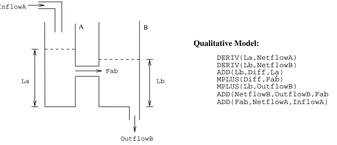
We consider identifying the qualitative model of the coupled-tanks system shown in Fig. 8. The measurable system variables are these: the input, InflowA, that pours into the top of tank A; the output,OutflowB, that pours out of the base of tank B; the flow of water from A to B,Fab; and the water-levelsLaandLb.
Qualitative Model:
,
ADD(NetflowB,OutflowB,Fab) ADD(Fab,NetflowA,InflowA) MPLUS(Lb,OutflowB) MPLUS(Diff,Fab) ADD(Lb,Diff,La) DERIV(Lb,NetflowB) DERIV(La,NetflowA) InflowA
A
Lb La
Fab
OutflowB B
Figure 8: A system comprised of two coupled tanks and its qualitative model.
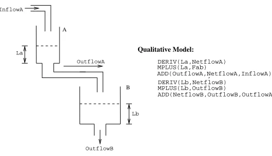
The coupled tanks system consists of two tanks connected together. This allows us to decompose the identification of this model into two stages. In the first stage, we focus on identifying a model for tank B, using the single tank system in Fig. 10 (often called the “bathtub” system in qualitative modelling literature). Any consistent models identified for the single tank system are then extended to return final models for the coupled tanks system (see Fig. 9).
B1 E1 B2 E2 ρ f
L
Coupled tank observations (with data from Tank A ignored)
Coupled tank observations (with data from both tanks)
QSIM constraints
Coupled tank model constraints General model constraints
Mode declarations QSIM constraints
Single tank model constraints General model constraints
Mode declarations {φ}
ρ f
L Single Tank
Models
Coupled Tank Models
A Bayes A Bayes
We note in passing that the final model for the coupled tanks is not simply a conjunction of two single tank models. This conjunction would not capture the fact that the flow from tank A to B is related to the difference in levels of fluid in A and B. The conjunction of the two models is, in fact, an appropriate model for the system of cascaded tanks shown in Fig. 11.
Qualitative Model:
Outflow L
Inflow
DERIV(L,Netflow)
ADD(Outflow,Netflow,Inflow) MPLUS(L,Outflow)
Figure 10: A single tank system with an input and output. The system variables are Inflow,
Outlflowand, L.
Qualitative Model: InflowA
, DERIV(La,NetflowA) A
B
OutflowB Lb La
OutflowA
MPLUS(La,Fab)
ADD(OutflowA,NetflowA,InflowA)
DERIV(Lb,NetflowB) MPLUS(Lb,OutflowB)
ADD(NetflowB,OutflowB,OutflowA)
Figure 11: A system comprised of two cascaded tanks. The qualitative model is simply a conjunc-tion of two single tank models.
We elaborate further on the elements in Fig. 9:
1. Background knowledge. This is comprised of the following components:
(a) Correct definitions of the QSIM constraints. Our definitions are based on those in Bratko (2001);
(c) Stage-specific constraints on the models constructed. This consists of specifying the number of qualitative constraints in the final model for each stage. This is 3 for Stage 1 (the single tank model) and 7 for Stage 2 (the coupled tanks model); and
(d) Stage-specific “mode” declarations similar to the description in Muggleton (1995) that provide domain and connectivity information for the qualitative variables (see Fig. 12);
2. Examples. These are in the form of qualitative states for the system variables. Recall that for the coupled tanks system these are: La, Lb, InflowA, Faband OutflowB(see Fig. 8). Clearly, flows and levels cannot be negative: we are further only interested in a system with a steady, non-negative input flow. That is, the only valid qualitative state for InflowA is
f low : 0...in f/std.OutflowB, on the other hand, can be any one of f low : 0/std, f low : 0/inc, f low : 0...in f/std, f low : 0...in f/inc, f low : 0...in f/dec. The level of waterLaorLbfor the system can similarly assume any of the following qualitative states: level : 0/std, level : 0/inc, level : 0...in f/std, level : 0...in f/inc, level : 0...in f/dec. Examples for Stage 1 ignore the
values observed for levels and flows for Tank A (that is,LaandInflowAare ignored: this can be easily specified using the mode declarations). Some observations for Stage 1 are shown in Fig. 13. Examples for Stage 2 contain the qualitative states of all the system variables.
3. Refinement operator and cost function. These are the operatorρAand fBayesdescribed earlier.
5.2 General Constraints on “Well-posed” Models
In Coghill et al. (2005), the term “well-posed” qualitative models is used to denote those models that satisfy a number of domain-independent constraints. We use the the following constraints from that report:2
1. Size. A well-posed model must be of a particular size (measured by the number of qualitative constraints).
2. Completeness. The model must contain all the measured variables.
3. Language. The number of instances of any qualitative constraint in a well-posed model should be below some prescribed number.
4. Sufficiency. The model must adequately explain the observed data. By “adequate”, we intend to acknowledge here that due to noise in the measurements, not all observations may be logical consequences of the model.3The percentage of observations that must be explainable in this sense is a user-defined value.
5. Redundant. The model must not contain relations that are redundant. For example, the rela-tionADD(Inflow,Outflow,X)is redundant if the model already hasADD(Outflow,Inflow,X).
2. This list excludes two constraints from the report: the “Determinate” constraint can be effectively enforced by the “Size” constraint. The “Connected” constraint that requires all intermediate variables should appear in at least two qualitative constraints is enforced by the more general “Irrelevant variables” constraint here. All the constraints are assumed to be encoded in the background knowledge for any given stage.
Modes:
DERIV(+level,-flow)
ADD(+level,+level,-level) ADD(+level,-level,+level) ADD(+flow,+flow,-flow) ADD(+flow,-flow,+flow) MPLUS(+level,-level) MPLUS(+level,-flow) MPLUS(+flow,-flow) MPLUS(+flow,-level) MMINUS(+level,-level) MMINUS(+level,-flow) MMINUS(+flow,-flow) MMINUS(+flow,-level) MINUS(+level,+level) MINUS(+flow,+flow)
A legal model:
MPLUS(L,Outflow) DERIV(L,Netflow)
ADD(Outflow,Netflow,Inflow)
Two illegal models:
MPLUS(L,Outflow) DERIV(L,Netflow) ADD(Outflow,L,Inflow)
(ADDcannot add flows to levels)
MPLUS(L,Outflow)
ADD(Netflow,Outflow,Inflow) DERIV(L,Netflow)
(ADDneedsNetflowto be known)
Figure 12: Example “mode” declarations for the qualitative constraints. For example, the mode declarationADD(+level,+level,-level)states that given values from domain “level” for the the first two arguments,ADDcomputes a value for the third argument (also from domain “level”). This is thus a simple form of dimensionality check. This prevents the ILP system from constructing model M2 (in which a variable from a “flow” domain is added to one from a “level” domain).
Fab OutflowB Lb
f low : 0...in f/std f low : 0/std level : 0/inc f low : 0...in f/std f low : 0...in f/inc level : 0...in f/inc f low : 0...in f/std f low : 0...in f/dec level : 0...in f/dec f low : 0...in f/std f low : 0...in f/std level : 0...in f/std
Figure 13: Some example observations of the relevant system variables for identification of a single tank model. No ordering is implied amongst these observations.
6. Contradictory. The model must not contain relations that are contradictory given other rela-tions present in the model.
7. Dimensional. The model must contain relations that respect the dimensionality of the vari-ables involved (this prevents, for example, constraints like ADD(Inflow,L,...) from ap-pearing in models for the single-tank system).
9. Causal. The model must be causally ordered (Iwasaki and Simon, 1986). In a simple sense, this requires a variable that appears on the right-hand side of a (qualitative) arithmetic con-traint should have appeared on the left-hand side of a conscon-traint earlier in the sequence.
The following constraints on the qualitative variables were also used. These are ad-hoc, but were nevertheless found to be extremely effective in constraining the space of possible models:
10. New variables. A well-posed model can contain no more than some prescribed number of new, or “hidden”, variables. Increasing this number usually increases the value of b in Remark 3 (this is equal to 1 for the single tank model: the hidden variable isNetflow).
11. Irrelevant variables. Variables in one constraint that are never used by another constraint are taken to be irrelevant. A well-posed model can contain no more than some prescribed number of irrelevant variables (this is equal to 0 for the single tank model).
12. Distinct variables. All variables in any constraint are distinct.
13. Dynamic variables. Well-posed models must includeDERIVconstraints for any pre-specified “dynamic” variables (these are variables that are known to change with time).
With these inputs, we summarise the results of using incremental model construction to identify a model for the coupled tanks system. Model construction proceeds in two stages. In the first stage, we attempt to identify a single tank model, by ignoring observations for levels and flows in tank A. Figure 14 shows the well-posed models identified by the system. The model with the lowest cost is extended in an attempt to identify a model for the coupled tanks system. Recall that the models selected from Stage 1 are subject to a limited form of generalisation before attempting to identify a model in Stage 2. The result of this generalisation step is shown in Figure 15. Each of these models are extended in Stage 2 to construct final models for the coupled tanks system: the results are in Fig. 16 (the fourth one is the correct model for the system).
Model No. Model Cost
1 MPLUS(Lb,OutflowB) −9.13
SUB(Fab,OutflowB,NetflowB) DERIV(Lb,NetflowB)
2 SUB(OutflowB,Fab,NetflowB) −5.37
MMINUS(Lb,E) DERIV(E,NetflowB)
3 SUB(Fab,OutflowB,NetflowB) −5.37
MPLUS(Lb,E) DERIV(E,NetflowB)
4 SUB(Fab,OutflowB,NetflowB) −5.37
DERIV(Lb,E) MPLUS(NetflowB,E)
5 SUB(Fab,OutflowB,NetflowB) −5.37
DERIV(Lb,E) MMINUS(NetflowB,E)
Model No. Model Model No. Model
1 MPLUS(Lb,OutflowB) 2 MPLUS(Lb,OutflowB)
SUB(Fab,OutflowB,NetflowB) SUB(Fab,OutflowB,NetflowB)
DERIV(Lb,NetflowB) DERIV(Lb,G)
3 MPLUS(Lb,F) 4 MPLUS(Lb,F)
SUB(Fab,OutflowB,NetflowB) SUB(Fab,OutflowB,NetflowB)
DERIV(Lb,NetflowB) DERIV(Lb,H)
5 MPLUS(Lb,F) SUB(Fab,F,NetFlowB) DERIV(Lb,NetFlowB)
Figure 15: Generalisations of the lowest cost model for the single tank system. These models are extended to identify models for the coupled tank system.
Model No. Model Model No. Model
1 MPLUS(Lb,OutflowB) 2 MPLUS(Lb,OutflowB)
SUB(Fab,OutflowB,NetflowB) SUB(Fab,OutflowB,NetflowB)
DERIV(Lb,NetflowB) DERIV(Lb,NetflowB)
SUB(InflowA,Fab,NetflowA) SUB(InflowA,Fab,NetflowA)
DERIV(La,NetflowA) DERIV(La,NetflowA)
ADD(OutflowB,NetflowA,H) ADD(NetflowB,NetflowA,H)
ADD(NetflowB,H,InflowA) ADD(OutflowB,H,InflowA)
3 MPLUS(Lb,OutflowB) 4 MPLUS(Lb,OutflowB)
SUB(Fab,OutflowB,NetflowB) SUB(Fab,OutflowB,NetflowB)
DERIV(Lb,NetflowB) DERIV(Lb,NetflowB)
SUB(InflowA,Fab,NetflowA) SUB(InflowA,Fab,NetflowA)
DERIV(La,NetflowA) DERIV(La,NetflowA)
MPLUS(InflowA,H) MPLUS(Fab,Diff)
MMINUS(InflowA,H) ADD(Lb,Diff,La)
5 MPLUS(Lb,OutflowB) SUB(Fab,OutflowB,NetflowB) DERIV(Lb,NetflowB) SUB(InflowA,Fab,NetflowA) DERIV(La,NetflowA) MPLUS(NetflowB,Diff) ADD(Lb,Diff,La)
Figure 16: Well-posed models identified for the coupled tank system. These were obtained by extending the lowest-cost model obtained for the single tank system in Fig. 14 (these are the first three constraints in all the models here). All models shown here have equal (lowest) cost. Model 4 is the target model
attempt to identify all seven constraints in a single stage (this is the “one-shot” approach); and (2)
Correct decomposition. The single tank model is identified in Stage 1, and then extended to the
coupled tank model in Stage 2. This resulted in the models in Figs. 14 and 16.
Figures 16 and 17 illustrate two points we wish to draw attention to about the procedure we have employed, namely:
1. The result may not be a unique model. For the identification of biological systems about which little is known, we do not see this as being a hindrance; and in many cases may even be preferable. New experiments could be proposed to discriminate between the models.
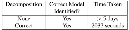
2. Decomposition can significantly increase the efficiency of system identification. No great significance should also be attached to the fact that the correct model is identified even with inappropriate decompositions—recall that the greedy search procedure employed is sub-optimal—although the robustness demonstrated is heartening, since in practice we may not be in a position to know the correct decomposition.
Decomposition Correct Model Time Taken Identified?
None Yes >5 days
Correct Yes 2037 seconds
Figure 17: The effect of decomposition on system identification. The ILP system without decom-position was halted after 5 days of execution.
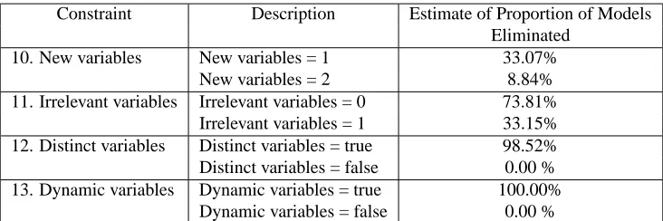
Finally, while most of the constraints 1–9 on posed models are motivated by some well-understood principles underlying qualitative reasoning, the constraints 10–13 on qualitative vari-ables are not. Figure 18 provides some empirical justification for the use of these constraints, by illustrating the proportion of a (uniform) random sample of 10,000 models, all of which satisfy constraints 1–9, but fail these constraints. Based on this proportion constraint 13 has the single strongest effect, followed by 12, 11, and 10.
6. Applications to Biological Systems
Constraint Description Estimate of Proportion of Models Eliminated
10. New variables New variables = 1 33.07%
New variables = 2 8.84%
11. Irrelevant variables Irrelevant variables = 0 73.81%
Irrelevant variables = 1 33.15%
12. Distinct variables Distinct variables = true 98.52% Distinct variables = false 0.00 % 13. Dynamic variables Dynamic variables = true 100.00%
Dynamic variables = false 0.00 %
Figure 18: Estimates of the reduction in the search space by the constraints introduced on qualita-tive variables. The last column represents the proportion of 10,000 models that satisfy the constraints 1–9 described in Coghill et al. (2005) but fail the corresponding con-straint in the second column.
the target qualitative model. The goal in each case is to examine if this target model is amongst the models identified by the ILP system. More details can be found in Section A.3.
6.1 Ecosystem-Level System Identification
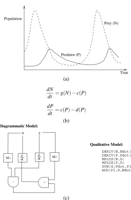
In this section we consider a problem in modelling the dynamics of populations. Specifically we are concerned with identification of a predator-prey model, following the description in Todorovski and Dˇzeroski (2001), which in turn is based on mathematical models developed for the same problem in Murray (1993).
The ecosystem considered is a simple one consisting of populations of predator and prey species—foxes and rabbits, say—that interact in the following manner. Assume that foxes only eat rabbits and that rabbits only eat grass, of which there is an unlimited supply. If the rabbit popu-lation is large, the fox popupopu-lation grows. In turn, many rabbits are eaten, resulting in a fall in their numbers. A smaller number of rabbits causes more foxes to die of starvation. Fewer foxes then causes an increase in the rabbit population, which leads to the entire cycle being repeated. This kind of oscillatory behaviour of the two populations is shown in Fig. 19(a). The dynamics of the popu-lations can be modelled using the Lotka-Volterra model, a variant of which is shown in Fig. 19(b). Under certain simplifying assumptions described, the qualitative model is in Fig. 19(c).
We examine reconstructing the model in Fig. 19(c) by using the incremental ILP system as a single-shot model constructor. For this, the ILP system is provided with: (a) the same background knowledge as in Section 5.1; (b) example observations of system behaviour generated using the target model in Fig. 19(c); and (c) the refinement operator and the Bayesian cost function described in Appendix A. The incremental search procedure commences with an empty model (by convention, denoted by /0) as the initial hypothesis (see Fig. 20).
Prey (N)
Predator (P)
Time Population
(a)
dN
dt =g(N)−c(P) dP
dt =c(P)−d(P)
(b)
M+ dtd dtd M+
− +
N
Qualitative Model:
DERIV(N,Ndot)
MPLUS(N,G) , MPLUS(P,D) SUB(G,Pdot,P1) ADD(P1,D,Ndot) Diagrammatic Model:
P
DERIV(P,Pdot)
(c)
Figure 19: Modelling predator-prey populations. The changes in populations are shown graphically in (a). There are two system variables: the predator population (P) and the prey popu-lation (N). At any given point in time, these variables satisfy the differential equation model in (b). This is a general form of the Lotka-Volterra model for population dynam-ics. The terms in the model are as follows: g(N) represents the growth-rate of the of the prey in the absence of predators; c(P)is the consumption rate of the predators; and
QSIM constraints
Predator−prey model constraints General model constraints
Mode declarations {φ}
ρ f
L Predator−prey
Models
A Bayes
Predator−prey observations
B E
Figure 20: Incremental model identification of predator prey models.
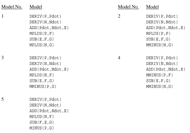
Model No. Model Model No. Model
1 DERIV(P,Pdot) 2 DERIV(P,Pdot)
DERIV(N,Ndot) DERIV(N,Ndot)
ADD(Pdot,Ndot,E) ADD(Pdot,Ndot,E)
MPLUS(P,F) MPLUS(P,F)
SUB(E,F,G) SUB(E,F,G)
MPLUS(N,G) MMINUS(N,G)
3 DERIV(P,Pdot) 4 DERIV(P,Pdot)
DERIV(N,Ndot) DERIV(N,Ndot)
ADD(Pdot,Ndot,E) ADD(Pdot,Ndot,E)
MPLUS(N,F) MMINUS(P,F)
SUB(E,F,G) SUB(E,F,G)
MMINUS(P,G) MMINUS(N,G)
5 DERIV(P,Pdot) DERIV(N,Ndot) ADD(Pdot,Ndot,E) MPLUS(N,F) SUB(F,E,G) MINUS(P,G)
Figure 21: Predator-prey models identified. The target model in Fig. 19(c) is Model 1.
6.2 Organ-Level System Identification
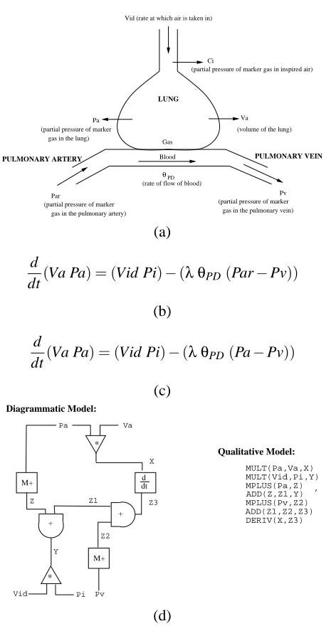
man-ner is shown in Fig. 22. The model is constructed using partial pressures of a measurable “marker” gas. A simplification of the model in Fig. 22(c) results from ignoring the blood vessels and treating the lung as a simple gas chamber as shown in Fig. 23(a). The resulting differential equation model is in Fig. 23(b) and the qualitative model is in Fig. 23(c).
We examine reconstructing a model for the lung by providing the ILP system with the approx-imate model Fig. 23(c): we are interested in investigating whether the ILP system can refine this to the model in Fig. 22(d). The ILP system is provided with: (a) the same background knowledge as in Section 5.1, with additional mode declarations needed for theMULT constraint; (b) example observations of system behaviour generated using the target model in Fig. 22(d); (c) the usual re-finement operator and cost function. The incremental search is provided with an intial hypothesis consisting of an approximate model for the lung:MULT(Va,Pa,F),MULT(Vid,Pi,G),DERIV(F,G)
(see Fig. 24).4
The results, shown in Fig.25, were obtained in 528 seconds of processor time. We note here that model identification required a generalisation of the approximate model provided (DERIV(F,G)is changed toDERIV(F,H)). Model 2 is the correct model.
6.3 Extra-Cellular System Identification
We use glucose-insulin balance in the human body as a third test case for incremental system iden-tification by ILP. Hormones are chemical messengers, usually small proteins, that play a regulatory role in an organism. Of these, the best known is probably insulin, the first protein whose structure was determined (the amino acid sequence, or primary structure, was determined in 1953 by Sanger and Tuppy). The role of insulin is primarily in maintaining the balance of glucose in the blood. Glucose is used as a source of energy by the central nervous system and by the muscles, and as a source of fat by adipose tissue and the liver, that stores it in the form of a starch called glycogen (see Fig. 26a). If the concentration of glucose in the blood rises too high (usually after digestion of food in the small intestine) then specialised cells in the pancreas are stimulated to produce insulin, by a process involving glycolysis (which we consider in the next section). The presence of insulin signals muscles, fat tissue and the liver to consume glucose, thus lowering it content in the blood. This lower amount of glucose in turn inhibits the production of insulin, and sugar levels rise again until a balance is achieved. This feedback process is not dissimilar to the functioning of a thermo-stat to maintain a constant temperature in a house. A model of this regulatory mechanism is shown in Fig. 26(b). The model is from Clancy and Kuipers (1994), and is based on a compartmental differential equation model developed by Ironi and Stefanneli (Ironi and Stefanelli, 1994).
Our goal is to reconstruct the qualitative model in Fig. 26(b) using by starting from the empty model. We examine identification of the full model in two stages: the first stage being concerned with identifying the insulin component (the first three constraints in the qualitative model) and the second, the glucose component (the remaining six constraints in the model). As before, the ILP sys-tem is equipped with: (a) QSIM relations and their definitions along with additional model-specific constraints; (b) example observatons of system behaviour using the target model in Fig. 26(b); and
Ci
Va
Par Pv
Blood Gas Vid (rate at which air is taken in)
(partial pressure of marker gas in inspired air)
LUNG
(volume of the lung) Pa
(partial pressure of marker gas in the lung)
(partial pressure of marker gas in the pulmonary artery)
(partial pressure of marker gas in the pulmonary vein) PULMONARY ARTERY PULMONARY VEIN
θPD
(rate of flow of blood)
(a)
d
dt(Va Pa) = (Vid Pi)−(λ θPD(Par−Pv))
(b)
d
dt(Va Pa) = (Vid Pi)−(λ θPD(Pa−Pv))
(c) * M+ + * Vid Pi M+ + d dt Pa Va Pv X Z3 Z2 Y Z1 Z Qualitative Model: MULT(Pa,Va,X) MULT(Vid,Pi,Y) MPLUS(Pa,Z) , ADD(Z,Z1,Y) MPLUS(Pv,Z2) ADD(Z1,Z2,Z3) DERIV(X,Z3) Diagrammatic Model: (d)
Figure 22: A model for the human lung. In this model, the marker gas is nitrous oxide. There are seven system variables: the rate of inspiration (Vid); the concentrations of the marker gas in the inspired air (Ci, which is taken to be proportional to the partial pressure Pi) and in the lung (Ca, proportional to the pressure Pa); the volume of the lung cavity (Va); the rate of flow of blood θPD; and the partial pressures in the artery Par and the vein Pv. On each inspiration, the variables satisfy the differential equation (b). The equation
(c) represents the same quantitative model with the assumption that Pa=Par, which is
Ci
Va Vid (rate at which air is taken in)
(concentration of marker gas in inspired air)
LUNG
(volume of the lung) Ca
(concentration of marker gas in the lung)
(a)
d
dt(Va Pa) = (Vid Pi)
(b)
d dt * *
Diagrammatic Model:
Pi
Pa Va
X
Y
Vid
Qualitative Model:
MULT(Va,Pa,X) MULT(Vid,Pi,Y) DERIV(X,Y) ,
(c)
QSIM constraints
Lung model constraints General model constraints
Mode declarations ρ f
L
Models
A Bayes
Lung observations
B E
Model
Approximate Lung Lung
Figure 24: Incremental model identification of lung models.
Model No. Model Model No. Model
1 MULT(Va,Pa,F) 2 MULT(Va,Pa,F)
MULT(Vid,Pi,G) MULT(Vid,Pi,G)
DERIV(F,H) DERIV(F,H)
SUB(Pv,Pa,J) SUB(Pv,Pa,J)
SUB(H,G,I) SUB(H,G,I)
MPLUS(I,J) MMINUS(I,J)
3 MULT(Va,Pa,F) 4 MULT(Va,Pa,F)
MULT(Vid,Pi,G) MULT(Vid,Pi,G)
DERIV(F,H) DERIV(F,H)
SUB(Pv,Pa,I) SUB(Pv,Pa,I)
SUB(H,I,J) SUB(H,I,J)
MPLUS(J,G) MMINUS(J,G)
Figure 25: Lung models identified, given the approximate model MULT(Va,Pa,F),
MULT(Vid,Pi,G),DERIV(F,G). The target model in Fig. 22(d) is Model 2.
(c) the refinement operator ρA and cost function fBayes. The full system identification process is
shown in Fig. 27.
Small Intestine
Glucose
Glucose
Central Nervous System
Insulin
Glucose
Glucose
Glucose Food
Pancreas Fat Tissue
Muscles
Liver
(a)
d dt M+
+
S+
M+
S+ + d dt
+
DI Iout
Iin
I
G
Gx
Ig
DG
Gout Gin
Qualitative Model:
DERIV(G,DG) SPLUS(G,Iin) MPLUS(G,Gx) SPLUS(I,Ig) MPLUS(I,Iout) DERIV(I,DI)
SUB(Iin,Iout,DI)
ADD(Gx,Ig,Gout) SUB(Gin,Gout,DG)
Diagrammatic Model:
(b)
Figure 26: Glucose regulation in the blood, shown pictorially in (a), and modelled qualitatively in (b). In the model,Gin refers to the glucose intake (in the form of food) andIin, the insulin produced by the pancreas.GandIare the glucose and insulin levels in the blood.
Gxis the insulin-independent consumption of glucose by the central nervous system and
Igthe insulin-dependent consumption of glucose by the muscles, fat tissue and the liver. The qualitative model in Clancy and Kuipers (1994) utilises a sigmoid functionSPLUS. For the model here, we use the standardMPLUSfunction, which is consistent with the original formulation in Ironi and Stefanelli (1994)
B1 E1 B2 E2
{φ}
ρ f L
Models
A Bayes
Models
A Bayes
ρ f L
QSIM constraints
Insulin model constraints General model constraints
Glucose−Insulin Insulin Stage
Glucose stage observations Insulin stage observations
QSIM constraints
Glucose model constraints General model constraints
Mode declarations Mode declarations
Figure 27: Incremental model identification of models for glucose regulation.
substantially more restrictive mode declarations than in other cases were needed to restrict the search space. Further, we restrict the search to occupy no more than 10,000 seconds of processor time. With these ad hoc constraints in place, we are able to repeat model identification using the two stages. The correct insulin model is obtained as before and the results after the glucose stage are shown in Fig.28. Model 3 is equivalent to the target model, given the equivalence ofSPLUSandMPLUSin experiments here.
6.4 Cell-Level System Identification
We use the glycolysis pathway as the final test case for incremental system identification by ILP. Glycolysis is the archetypal pathway. It was historically one of the first to be unravelled, with Otto Meyerhof winning the Nobel prize for discovering key steps in it. Specifically, Meyerhof and col-leagues “. . . were unusually accomplished in breaking down glycolysis into its many separate com-ponents, analysing each step separately, then reassembling the constituent parts within an overall system.”5 Glycolysis still presents a challenge to model accurately. The special interest here is that it is significantly different in nature to the models considered so far in the paper, which have all been abstractions of ordinary differential equations. We examine now how the qualitative representation language could be used to develop other kinds of models.
Our qualitative model for glycolysis uses 15 metabolites, namely: pyruvate (pv), glucose (glc), phosphoenolpyruvate (pep), fructose 6-phosphate (f6p), glucose 6-phosphate (g6p), dihydroxyace-tone phosphate (dhap), 3-phosphoglycerate (3pg), 1,3-bisphos phoglycerate (1,3bpg), fructose 1,6-biphosphate (f16bp), 2-phosphoglycerate (2pg), glyceraldehyde 3-phosphate (g3p), ADP (adp), ATP (atp), NAD (nad), and NADH (nadh). We have not included H+, H2O, or Orthophosphate as they are assumed to be ubiquitous. The set of reactions in the pathway are shown in Fig. 29.
We will use the following simple qualitative model for enzymes and metabolites. Metabolites are qualitative variables, whose domains are defined by the name of the metabolite and the land-marks 0 and in f . Qualitative states of the metabolites are restricted to 0/std,0...in f/std, 0...in f/inc,
0...in f/dec. A “qualitative cell-state” is given by the qualitative states of the metabolites of
inter-est in the cell. Enzymes are associated with “qualitative reactions”, which result in a qualitative
Model No. Model Model No. Model
1 DERIV(I,DI) 2 DERIV(I,DI)
MPLUS(I,Iout) MPLUS(I,Iout)
SUB(Iin,Iout,DI) SUB(Iin,Iout,DI)
DERIV(G,DG) DERIV(G,DG)
MPLUS(G,Iin) MPLUS(G,Iin)
SPLUS(G,Gx) SPLUS(G,Gx)
ADD(I,Gx,I1) ADD(Iout,Gx,I1)
SPLUS(I1,J) SPLUS(I1,J)
SUB(Gin,J,DG) SUB(Gin,J,DG)
3 DERIV(I,DI) 4 DERIV(I,DI)
MPLUS(I,Iout) MPLUS(I,Iout)
SUB(Iin,Iout,DI) SUB(Iin,Iout,DI)
DERIV(G,DG) DERIV(G,DG)
MPLUS(G,Iin) MPLUS(G,Iin)
SPLUS(G,Gx) SPLUS(G,Gx)
SPLUS(I,Ig) MMINUS(I,Ig)
ADD(Gx,Ig,Gout) ADD(Gin,Ig,J)
SUB(Gin,Gout,DG) SUB(J,Gx,DG)
5 DERIV(I,DI) DERIV(I,Iout) SUB(Iin,Iout,DI) DERIV(G,DG) MPLUS(G,Iin) SPLUS(I,Ig) ADD(G,Ig,G1) SPLUS(G1,Gout) SUB(Gin,Gout,DG)
Figure 28: Models for glucose-insulin regulation. The target model is Model 3.
decrease in the amounts of the reactants and a qualitative increase in the amounts of the products. Examples of each of these are in Fig. 30.
We are interested here in finding a sequence of qualitative reactions that are consistent with the qualitative cell-states before and after glycolysis. For this, we introduce aPATHWAYrelation which, for a given sequence of qualitative reactions, holds for pairs of qualitative cell-stateshBe f ore,A f teri such that the qualitative state of each metabolite in Be f ore can be transformed into its state in A f ter by the qualitative reactions. With this relation, the 3 stage glycolysis process can be modelled as shown in Fig. 31. The reader will note that in this model, reactions proceed sequentially. Of course, biologically speaking, this is not how things happen: reactions that can proceed, do so concurrently. While this can be modelled using a slightly different definition for thePATHWAYrelation, the model used here is simpler. There are also good historical reasons to adopt this simpler approach. Gly-colsis, as the quote above makes clear, and indeed most other pathways have been uncovered by first experimentally separating them into constituent parts (the qualitative modelling of pathways in (King et al., 2005) did not make this assumption, making the resulting models both difficult to identify—all reactions had to be identified in one-shot—and inefficient to execute).
1. (Hexokinase): glucose + ATP⇔glucose 6-phosphate + ADP.
2. (Phosphoglucose isomerase): glucose 6-phosphate⇔fructose 6-phosphate. 3. (Phosphofructokinase): fructose 6-phosphate + ATP
⇔fructose 1,6-biphosphate + ADP. 4. (Aldolase): fructose 1,6-biphosphate
⇔dihydroxyacetone phosphate + glyceraldehyde 3-phosphate. 5. (Triose phosphate isomerase): dihydroxyacetone phosphate
⇔glyceraldehyde 3-phosphate. 6. (Glyceraldehyde 3-phosphate dehydrogenase):
glyceraldehyde 3-phosphate + NAD⇔1,3-bisphosphoglycerate + NADH. 7. (Phosphoglycerate kinase): 1,3-bisphosphoglycerate + ADP
⇔3-phosphoglycerate + ATP. 8. (Phosphoglycerate mutase): 3-phosphoglycerate⇔2-phosglycerate. 9. (Enolase): 2-phosphoglycerate⇔phospoenolpyruvate.
10. (Pyruvate kinase): phospoenolpyruvate + ADP⇔pyruvate + ATP.
Figure 29: The reactions comprising the glycolysis pathway. The reactions that consume ATP and NADH are not explicitly included. Glycolysis proceeds in three stages: primary (re-actions 1–3), splitting (re(re-actions 4 and 5) and phosphorylation (re(re-actions 6–10). The enzymes involved are in parentheses.
Qualitative states of some metabolites
at p : 0...in f/std, dhap : 0/std, nad : 0...in f/dec
A qualitative cell-state
{ad p : 0/std,at p : 0...in f/std,f 16bp : 0/std,f 6p : 0/std,g6p : 0/std,glc : 0...in f/std}
A qualitative reaction glc+at p g6p+ad p
Some cell-states consistent with glc+at p g6p+ad p
Before:{ad p : 0/std,at p : 0...in f/std,f 16bp : 0/std,f 6p : 0/std,g6p : 0/std,glc : 0...in f/std}
After: {ad p : 0...in f/inc,at p : 0...in f/dec,f 16bp : 0/std,f 6p : 0/std,g6p : 0...in f/inc,glc : 0...in f/dec} After: {ad p : 0...in f/inc,at p : 0/std,f 16bp : 0/std,f 6p : 0/std,g6p : 0...in f/inc,glc : 0...in f/dec}
Figure 30: Examples of the qualitative representation used for metabolites, cell-states and chemical reactions. In this, a qualitative reaction causes a qualitative decrease in the reactants and a qualitative increase in the products. The non-determinate nature of qualitative arithmetic means that a cell can be in one of several different states after a reaction.
more than 5 reactions are allowed in a pathway; reactions must use all the metabolites; and reactions have to satisfy some basic constraints of chemical feasibility.6 In addition, the background knowl-edge contains an additional constraint that ensures that the model proposed is of the sequential form shown; (b) examples of system behaviour generated using the target model; and (c) the usual re-finement operator and cost function. The incremental search procedure commences with the empty model /0as the initial hypothesis (see Fig. 32).
GLYCOLYSIS(Be f ore,A f ter) if
PATHWAY(Be f ore,S1,hat p+glc ad p+g6p,g6p f 6p,at p+f 6p ad p+f 16bpi)
PATHWAY(S1,S2,hf 16bp dhap+g3p,dhap g3pi)
PATHWAY(S2,A f ter,hg3p+nad 1,3bpg+nadh,1,3bpg+ad p 3pg+at p,
3pg 2pg,2pg pep,ad p+pep at p+pvi) where:
PATHWAY(S,F,hR1,R2, . . .Rni)
i=0, S0=S
for i=1. . .n
QREACTION(Si−1,Ri,Si)
F=Sn
QREACTION(State,R,NewState)
QDECREASE(State,Reactants(R),S)
QINCREASE(S,Products(R),NewState)
Figure 31: A qualitative model for glycolysis. Pathways consist of qualitative reactions, each of which result in a qualitative decrease in the reactants and a qualitative increase in the products. The non-determinacy of qualitative arithmetic means that a qualitative re-action acting on a cell-state could result in one of several new cell-states (since there would be several ways to decrease or increase the qualitative values of metabolites). The system identification task is to find the definition forGLYCOLYSISgiven definitions forPATHWAY,QREACTION,QDECREASEandQINCREASE.
B1 E1 B2 E2 B3 E3
{φ} ρ f L Models A Bayes Models A Bayes ρ f L Glycolysis Models A Bayes QSIM constraints
Priming model constraints General model constraints
Splitting Stage Priming Stage
Splitting stage observations Priming stage observations
ρ f
L
Feasible reactions constraints PATHWAY definition Mode declarations
QSIM constraints
Splitting model constraints General model constraints
Feasible reactions constraints
Mode declarations
Phosphorylation stage observations QSIM constraints
Phosphorylation model constraints General model constraints
Feasible reactions constraints PATHWAY definition
Mode declarations PATHWAY definition
Figure 32: Incremental model identification of models for glycolysis.