Multi-Agent Reinforcement Learning in Common Interest and Fixed Sum Stochastic Games: An Experimental Study

(1)

Multi-Agent Reinforcement Learning in Common Interest and Fixed

Sum Stochastic Games: An Experimental Study

∗

Avraham Bab [email protected]

Ronen I. Brafman [email protected]

Department of Computer Science Ben-Gurion University

Beer-Sheva 84105, Israel

Editor: Michael Littman

Abstract

Multi Agent Reinforcement Learning (MARL) has received continually growing attention in the past decade. Many algorithms that vary in their approaches to the different subtasks of MARL have been developed. However, the theoretical convergence results for these algorithms do not give a clue as to their practical performance nor supply insights to the dynamics of the learning process itself. This work is a comprehensive empirical study conducted on MGS, a simulation system de-veloped for this purpose. It surveys the important algorithms in the field, demonstrates the strengths and weaknesses of the different approaches to MARL through application of FriendQ, OAL, WoLF, FoeQ, Rmax, and other algorithms to a variety of fully cooperative and fully competitive domains in self and heterogeneous play, and supplies an informal analysis of the resulting learning processes. The results can aid in the design of new learning algorithms, in matching existing algorithms to specific tasks, and may guide further research and formal analysis of the learning processes.

Keywords: reinforcement learning, multi-agent reinforcement learning, stochastic games

1. Introduction

Multi-Agent Reinforcement Learning (MARL) deals with the problem of learning to behave well through trial and error interaction within a multi-agent dynamics environment when the environ-mental dynamic and the algorithms employed by the other agents are initially unknown. Potential applications of MARL range from load balancing in networks (Schaerf et al., 1995) and e-commerce (Sridharan and Tesauro, 2000) to planetary exploration by mobile robot teams (Zheng et al., 2006). MARL adopts the game theory model of a Stochastic (a.k.a. Markov) Game (SG) to model

the multi-agent-environment interaction. The non-cooperative1game theoretic solution concept for

SGs is the Nash Equilibrium (NE). A NE is a behavioral profile, namely a set of decision rules, or policies, for all agents, such that no agent can benefit from unilaterally changing its behavior. However, SGs may have multiple NEs with different values, none of which is necessarily strictly optimal (i.e., preferable by all agents to all other NEs). Thus, in the general case, it is not clear which behavior should be considered “optimal,” even when the environmental dynamics and the other players’ set of possible strategies are known. For this reason, development of MARL algorithms

∗. A preliminary version of this paper that covered some of the results on common-interest games appeared in Bab and Brafman (2004).

(2)

has concentrated on algorithms for classes of SGs in which there is a unique NE, or in which all NEs have the same value. In such cases, it is possible to measure the performance of learning algorithms

against a well defined target.2 In particular, most MARL algorithms are shown to converge to such

NEs in self play in either Common Interest SGs (CISGs) or Fixed Sum SGs (FSSGs), which we describe next.

CISGs model environments in which the agents share common interests and have no conflicting interests. In such environments, defining an optimal joint behavior for all agents is straightforward— it is the joint behavior that maximizes the common interests. However, since the agents are inde-pendent, they face the task of coordinating such joint behavior in the case in which there are several optimal options. FSSGs, on the other hand, model environments in which two agents have fully conflicting interests. In FSSGs, there is a well defined minimax solution (Filar and Vrieze, 1997).

Several different MARL algorithms have been proved to converge in the limit to optimal behav-ior in CISGs (Littman, 2001; Wang and Sandholm, 2002) and in FSSGs (Littman, 1994). One has

been shown to converge toε-optimal behavior in polynomial time in both CISGs and FSSGs

(Braf-man and Tennenholtz, 2002, 2003). Since MARL is, by its nature, an online task, determining the abilities of the algorithms in practical domains is important. However, existing theoretical results

tell us very little about the practical efficacy of the algorithms;3 to this end a comprehensive

em-pirical comparison is necessary. Experimental results that have been published in the literature on CISGs (Claus and Boutilier, 1997; Wang and Sandholm, 2002; Chalkiadakis and Boutilier, 2003) and on FSSGs (Littman, 1994; Uther and Veloso, 2003; Bowling and Veloso, 2002), do not meet this demand. They do not examine representative samples of algorithms and/or use small and simple test models and/or do not examine online learning. Furthermore, the different experimental setups used in different publications do not enable cross comparisons of the algorithms they examine.

This work provides a comprehensive empirical study of MARL algorithms in CISGs and FSSGs. It offers a decomposition of the MARL task into subtasks. It then compares three algorithms for learning in CISGs: FriendQ (Littman, 2001), OAL (Wang and Sandholm, 2002), and Rmax (Braf-man and Tennenholtz, 2002); and three algorithms for learning in FSSGs: FoeQ (Litt(Braf-man, 1994, 2001), WoLF (Bowling and Veloso, 2002) and Rmax (Brafman and Tennenholtz, 2002). These algorithms were selected because they represent a variety of approaches to the offered subtasks, while providing certain convergence guarantees. We experimented with diverse variants of these algorithms on several non-trivial test environments which we designed to demonstrate the efficacy of the different approaches in each of the subtasks. To concentrate attention on the basic learning task, full state observability and perfect monitoring (that is, the ability to observe the actions of other agents) are assumed. The results allow us to rank the performance of the algorithms according to properties of the environment and possible performance measures.

The experiments for this work have been conducted using MGS, a Markov Game Simulation system developed for this purpose. MGS is implemented in the Java programming language and supplies interfaces and abstract classes for the simple creation of players and grid worlds and con-venient logging. We believe that MGS can be of good service to both MARL algorithm designers

and users. MGS is free, open source software available athttp://www.cs.bgu.ac.il/˜mal.

2. Much recent work is concerned with the question of how to define and evaluate the performance of learning algo-rithms in more general games. See, for example, Vohraa and Wellman (2007) which is devoted to this issue. 3. Vidal and Durfee (2003) take a step towards theoretical analysis of the learning dynamics. They offer theoretical

(3)

The paper is organized as follows. Necessary background is given in Section 2. Sections 3 and 4 describe the particular problems and algorithms for CISGs and FSSGs, respectively, and present experimental results and analysis. Section 5 describes MGS and Section 6 concludes the paper.

2. Multi-Agent Reinforcement Learning and Stochastic Games

Multi-Agent Reinforcement Learning (MARL) is an extension of RL (Sutton and Barto, 1998; Kaelbling et al., 1996) to multi-agent environments. It deals with the problems associated with the learning of optimal behavior from the point of view of an agent acting in a multi-agent en-vironment. At the outset, the environmental dynamics and the algorithms employed by the other players are unknown to the given agent. The environment is modeled by a finite set of states and the agents-environment interaction is discretized into time steps. At each time step, the players simultaneously choose actions, available from individual sets of actions. Depending stochastically on the joint action, the environment transitions into its next state and each player is rewarded. The present work assumes full state observability and perfect monitoring, namely, the agent observes the actions taken and rewards received by the other players. It also assumes that the agents have no additional means of communication. The multi-agent-environment interaction is modeled by a Stochastic (a.k.a Markov) Game (SG).

Definition 2.1 (Stochastic Game) An SG G :={α,A,S,T,R}consists of:

• α={1, ...,n}- a set of players. We will typically use n to denote the number of players.

• A=A1×A2×...×An– a set of joint actions. Aiis a set of private actions available to player

i.

• S - a set of states.

• T : S×A×S→[0,1]- a transition function. T(s,a,s0) =Pr(s0|s,a)is the probability that the system transitions to state s0when joint action a is taken at state s (∑_s0T(s,a,s0) =1).

• R : S×A×S→Rn- a payoff function. [R(s,a,s0)]iis i’s reward upon transition from state s

to state s0under joint action a.

The behavior of player i in an SG is described by a policy. A policy is a mapping πi:H →

P D₍_A_i₎_whereH _:₌_{₍_s₀_,_a₁_,_s₁_,_a₂_{, ...,}_s_j₎_| _j_≥₀_}_{is the set of possible histories of the process}

andP D₍_A_i₎_{is a probability distribution over A}_i_{. A policy that depends only on the current state}

of the process, that is, πi : S→P D(Ai) is called stationary. A deterministic policy, that is a

mapping, πi :H →Ai is called pure, whereas a stochastic policy is called mixed. A tuple of

policiesπ= (π1, . . . ,πn)for n players of a SG is called a policy profile. The objective of an agent in a SG is to maximize some function of its accumulated payoffs, referred to as the agent’s return. In this study, the infinite horizon discounted return (IHDR) is considered. The expected IHDR for player i, resulting from policy profileπ, is defined by the sum∑_t∞₌₀γtEπ(ri_t)where r_ti is player i’s payoff at time t andγ∈[0,1)is a discount factor. Consequently, a state-policy value function, V is defined by Vi(s,π) =∑∞t=0γtEπ(rti|s0=s).

(4)

maximize different natural objectives. While we use formulations that aim to maximize IHDR, the games we experiment on are such that any good policy will reach an absorbing state (following which the agents are placed in their initial states) quickly. In this setting, given a reasonably high

discount factor, γ, IHDR maximizing behavior will be identical to behavior maximizing average

reward. Consequently, we will sometimes find it more natural to report performance measures such as average reward per step.

For single agent domains, where n=1, there is always an optimal pure stationary policy that

maximizes V(s,π)for all s∈S (Filar and Vrieze, 1997). The single-agent state-policy value function

for the optimal policy, referred to as the state-value function, is the unique fixed point of the Bellman optimality equations

V∗(s) =max

a∈A R(s,a) +γ_s

∑

0_∈_S

T(s,a,s0)V∗(s0)

!

,∀s∈S.

An optimal policy may be specified byπ∗(s) =arg maxa∈A(R(s,a) +γ∑s0_∈_ST(s,a,s0)V∗(s0)) (Put-erman, 1994). Many single agent Reinforcement Learning (RL) methods interleave approximation of the value function with derivation of a learning policy from the current approximation.

In MARL, maximizing the IHDR cannot be done by simply maximizing over (private) policies since the return depends also on the other players’ policies which, in turn, may depend on the agent’s actions. Hence, to maximize the IHDR, the agent must adopt a policy that is a best response to the other players’ policies. Formally, πi is a best response toπ−i= (π1, ...,πi−1,πi+1, ...,πn) if

Vi(s,π1, ...,πi, ...,πn)≥Vi(s,π1, ...,π0i, ...,πn)for allπ0iand s∈S. A best response function is defined by BR(π−i) =

πi|πiis a best response toπ−i . In general,T_π−iBR(π−i) =/0, namely, there is no policy that is a best response to all of the possible behaviors of the other players.

Whereas the goal of single-agent reinforcement learning is clear—maximizes some aggregate of your reward stream, the picture is more complex in multi-agent settings. Here, one’s performance depends on what the other agents do, and strategic considerations come to the fore. For instance, the well-known notion of Nash Equilibria does not, in general, provide a clear target for learning algorithms, as many such equilibria may exist in a game, none of which dominates the others. Although some recent work has attempted to clarify this issue (Brafman and Tennenholtz, 2004; Shoham et al., 2007), there is still no clear agreement on the goal of MARL. However, there are two special classes of SGs in which there is a clear target for learning: Common-interest SGs, and Fixed-sum SGs. These are two extreme cases of SGs where players are either fully cooperative or fully opposed. Much work in the area of MARL has concentrated on these classes of SGs, and algorithms with good theoretical guarantees exist for each of them. In this paper, we analyze a number of algorithms for such games.

3. Learning in CISGs

In CISGs, the payoffs are identical for all agents. That is, for any given choice of s,a and s0 and

(5)

select a particular joint action. On the other hand, CISGs do not require that agents confront the more difficult task of optimizing behavior against an adversary.

For efficient learning in CISGs, agents are required to coordinate on two levels: (i) select whether to explore or exploit in unison; and (ii) coordinate the exploration and exploitation moves. This requirement stems from the dependence of the team’s next state on the actions of all its mem-bers. Hence, it is impossible for the team to exploit unless all agents exploit together, and using the same choice of exploitation strategy. Exploration, too, can be less effective when only some agents explore.

Furthermore, even when the model is known, multiple NEs yielding maximal payoffs to the agents are likely to exist, and the agents still face the task of reaching consensus on which specific NE to play.

This section describes and compares three algorithms for learning in CISGs: OAL (Wang and Sandholm, 2002), FriendQ (Littman, 2001), and Rmax (Brafman and Tennenholtz, 2002). They were selected because each embodies a different approach to learning, while guaranteeing conver-gence to optimal behavior in CISGs. Diverse variants of these algorithms are examined with the aim of gaining better understanding of their performance with respect to their approach to

exploration-exploitation, information propagation, and coordination tasks.4 These variants and the tasks on

which they were tested are described in the following subsections.

3.1 FriendQ

FriendQ (Littman, 2001) extends single agent Q-learning into CISGs. After taking a joint action a= (a1, ...,an) in state s at time t and reaching state s0 with reward rcur, each agent updates its

Q-value estimates forhs,aias follows:

Qt(s,a)←(1−αt)Qt−1(s,a) +αt

rcur+γmax

a0_∈_AQ(s

0_,_a0₎

.

As in single agent Q-learning, given that ∑∞_t₌₀αt =∞,∑∞t=0α2t <∞and that every joint action is performed infinitely often in every state, the Q-values are guaranteed to converge asymptotically to

Q∗ (Littman, 2001). Convergence to optimal behavior is achieved using Greedy in the Limit with

Infinite Exploration Learning Policies (GLIELP) (Sutton and Barto, 1998).

There are two types of GLIELPs, directed and undirected. Directed GLIELPs reason about the uncertainty of the current belief about action values (Kaelbling, 1993; Dearden et al., 1998, 1999; Chalkiadakis and Boutilier, 2003). However, the computational complexity of the underlying statistical methods makes directed exploration impractical for simulations of the size conducted in

this study.5 Two popular undirected exploration methods areε-greedy action selection and Boltzman

distributed action selection. There is no established technique for applying Boltzman exploration to

FriendQ, so in our experiments it is executed withε-greedy exploration only.ε-greedy exploration

is applied to SGs in the following way: each agent randomly picks an exploratory private action

with probabilityε, and with probability 1−εtakes its part of an optimal (greedy) joint action with

4. By this we mean the ability of the algorithm to propagate information observed in one state to other states. For example, Q-learning does not propagate information beyond the current state, unless techniques such as eligibility traces are used.

(6)

respect to the current Q-value (Claus and Boutilier, 1997). εis asymptotically decreased to zero over time.

Since full state observability, perfect monitoring, and identical initial Q-values to all agents are assumed, all agents maintain identical Q-values throughout the process, and consequently the same classification of greedy actions. But, two problems arise: (i) Because randomization is used to select exploration or exploitation, the agents cannot coordinate their choice of when and what to explore. (ii) In the case of multiple optimal policies, that is, several joint actions with maximal Q-values in a certain state, the agents must agree on one such action. The original FriendQ algorithm has no explicit mechanism for handling these issues.

This work compares some enhanced versions of FriendQ: First, Uncoordinated FriendQ (UFQ), the simple version described above, is tested. Next, the effect of adding coordination of greedy joint actions by using techniques introduced by Brafman and Tennenholtz (2003) is examined. Basically, a shared order over joint actions is used for selecting among equivalent NEs. If such an order is not built into the agents, it is established during a preliminary phase using an existing technique (Brafman and Tennenholtz, 2003). This version is referred to as Coordinated FriendQ (CFQ). Then, coordination of exploration and exploratory actions is added in Deterministic FriendQ (DFQ). In DFQ, the agents explore and exploit in unison, always exploring the least tried joint action. An

exploratory action is taken each b1/εc0th move. Finally, we add Eligibility Traces (Sutton and

Barto, 1998) to DFQ (ETDFQ).6Eligibility Traces propagate new experience to update Q-values of

previously visited states and not only the most recently visited state.

3.2 OAL

OAL combines classic model-based reinforcement learning with a new fictitious play algorithm for action and equilibrium selection named BAP (Biased Adaptive Play) (Wang and Sandholm, 2002). BAP is an action-selection method for a class of repeated games that contains common interest games. Here, BAP is described in the context of common interest repeated games. Let m and k

be integers such that 1≤k≤m. Each agent maintains a memory of the past m joint actions. At

the first m steps of the repeated game, each player randomly chooses its actions. Starting from step

m+1, each agent randomly samples k out of the m most recent joint actions. Let SPibe the set of k

joint actions drawn by agent i at some time step. If (i) there is a joint action a0that is estimated to

beε-optimal, such that for all a∈SPi, a−i⊂a0(where a−i⊂a0denotes the fact that the individual actions of all agents other than agent i are identical in a and a0), and (ii) there is at least one optimal joint action a∈SPi, then agent i chooses its part of the most recent optimal joint action in SPi. If

the above two conditions are not met, then agent i chooses an action ai that maximizes its expected

payoff under the assumption that the other players’ sampled history reflects their future behavior. This type of action selection is known as fictitious play (Brown, 1951).

EP(ai) =

∑

a−i_∈_SP

i

R(ai∪a−i)

N(a−i,SPi)

k

where N(a−i,SPi)is the number of occurrences of a−iin SPi. Given that there is no sub-optimal NE

and m≥k(n+2), BAP is guaranteed to converge to a NE. It was shown that, for every game that

satisfies these conditions, there is some positive probability p and some positive integer T such that

(7)

for any history of plays, with probability at least p, BAP converges to a consensus in T steps. That is, all players agree in the same joint-action which is a NE.

After observing a transition from state s on action a, OAL updates Q-values according to the learning rule

Qt+1(s,a) =Rt(s,a) +γ

∑

s0

Tt(s,a,s0)max

a0 Qt(s

0_,_a0₎

where Rt, the approximated mean reward, and Tt, the approximated transition probability are

esti-mated using the statistics gathered up to time t. At each step, OAL constructs a Virtual Game (VG) for the current state-game (the matrix game defined by the current state’s Q-values) and plays ac-cording to it. The VG has common payoff 1 for any optimal joint action and payoff 0 for any other

action. In our implementation we use the VG in conjunction withε-greedy as well as Boltzman

action selection. Boltzman action selection is implemented as follows: At each step, an action is sampled according to the Boltzman distribution induced by the Expected Payoffs in the current VG

eEP(s,a)/τ

∑beEP(s,b)/τ

.

If a sub-optimal action is sampled, it is explored by the agent, otherwise BAP is executed on the VG to select an exploitation action.

We examine OAL also with an addition of Prioritized Sweeping (PS) (Moore and Atkeson, 1993) to the underlying Q-learning algorithm (PSOAL). PS is a heuristic method for optimizing finite propagation of TD-errors in the model. PS attempts to order propagation according to the size of the change to the Q-values, for example, states that are liable to have a greater update should be updated first. For comparison, a combination of the model-based Q-learning algorithm used by OAL with the action and equilibrium-selection technique used by CFQ is also examined. This combination is referred to as ModelQ (MQ).

3.3 Rmax

Rmax (Brafman and Tennenholtz, 2002) is a model-based algorithm designed to handle learning in MDPs and in fixed-sum stochastic games. However, because Rmax does not make random decisions (e.g., random exploration), its MDP version can also be used to tackle MARL in CISGs. Brafman and Tennenholtz (2003) view a CISG as an MDP controlled by a distributed team of agents and show how such a team can coordinate its behavior given a deterministic algorithm such as Rmax. In a preliminary phase of the game, a protocol is used to establish common knowledge of the individual action sets, of orders over these sets, and of an order over the agents. At each point in time, all agents have an identical model of the environment and know what joint action needs to be executed next (when a number of actions are optimal with respect to the current state, the agents use the shared order over joint actions to select among these actions). Thus, each agent plays its part of this action. It is shown that even weaker coordination devices can be used, and that these ideas can be employed even under imperfect monitoring.

Rmax maintains a model of the environment, initialized in a particular optimistic manner. It always behaves optimally with respect to its current model, while updating this model (and hence

its behavior) when new observations are made. The model M0used by Rmax consists of n+1 states

S0 ={s0, ...,sn}where s1, ...,sn correspond to the states of the real model M, and s0is a fictitious

state.7 _{The transition probabilities in M}0 _{are initialized to T}

M0(s,a,s₀) =1 ∀hs,ai ∈S0×A. The

(8)

reward function is initialized to RM0(s,a) =R_max∀hs,ai ∈S0×A, where R_maxis an upper bound on maxs∈S,a∈AR(s,a). Each state/joint-action pair in M0 is classified either as known or as unknown. Initially, all entries are unknown.

Rmax computes an optimal policy with respect to M0 and follows this policy until some entry

becomes known. It keeps the following records: (i) number of times each action was taken at each state and the resulting state; (ii) the actual rewards, rac(s,a), received at each entry. An entry(s,a) becomes known after it has been sampled K1 times, such that with high probability TM(s,a,s0)−ρ≤

PE(s,a,s0|K1)≤TM(s,a,s0) +ρ where TM is the transition function in M, PE(s,a,· |K1) is the

empirical transition probability according to the K1 samples, andρis the accuracy required from M0.

When an entry(s,a)becomes known, the following updates are made: TM0(s,a,·)←PE(s,a,· |K1) and RM0(s,a)←r_ac(s,a). Then, a new deterministic optimal policy with respect to the updated

model is computed and followed. Rmax converges to anε-optimal policy in polynomial number of

steps.

The worst-case bounds on K1 (Brafman and Tennenholtz, 2002) assume maximal entropy on the transition probabilities, that is, TM(s,a,s0) =1/|S|for all s,a,s0. These bounds, although polyno-mial, are impractical. In the experiments, these bounds are violated, which enables us to eliminate

knowledge of the state space size. Furthermore, Rmax is not assumed to be known. Instead, it is

initialized to some positive value and updated online to be twice the highest reward encountered so far.

3.4 Discussion of Algorithms

Returning to the FriendQ algorithm, the efficiency of GLIELPs depends on the topology and dy-namic of the environment. If the probability to explore falls low before “profitable” parts of the environment are sufficiently sampled, the increasing bias to exploit may keep the agents in sub-optimal states. As a result, GLIELPs can exhibit significant differences depending on the particular schedule of exploration. In model free algorithms, and FriendQ, in particular, this phenomenon is intensified by the decreasing learning rate that makes learning from the same experience slower over time. GLIELPs also suffer from their inability to completely stop exploration at some point. Thus, even when greedy behavior is optimal, the agent is unable to attain optimal return.

The exploration method of Rmax is less susceptible to the structure of the environment. As long

as Rmax cannot achieve actual returnε-close to optimal, it will have a strong bias for exploration

since unknown entries seem very attractive. This strategy is profitable when the model can be learned in a short time. However, the theoretical worst-case bounds for convergence in Rmax are impractical. In practice, much lower values of K1 suffice. Bayesian exploration (Dearden et al., 1999; Chalkiadakis and Boutilier, 2003) and locality considerations might help to obtain better adaptive bounds, but these approaches are not pursued here.

GLIELPs make learning “slower” as the agents get “older”. To accelerate learning, an algorithm can try to use new experience in a more exhaustive manner, using it to improve behavior in previ-ously visited states. Eligibility traces are used to propagate information in FriendQ. In model-based algorithms, an exhaustive computation per new experience is too expensive (in CPU time). Thus, OAL is tested with Prioritized Sweeping and Rmax makes one exhaustive computation each time a new entry becomes known (and does no further computation).

(9)

have no element (private action) of some optimal joint action have a lower chance of being ex-plored. Hence, some popular techniques for decreasing exploration in the single agent case lead to

finite exploration in the multi agent case. For example, takingε=1/time forε-greedy policies will

make the chance of exploring such joint actions 1/timen, where n is the number of agents.

Equilibrium selection in Rmax and CFQ comes with no cost. In OAL, it is essentially a random protocol for achieving consensus. This protocol may take long to reach consensus with respect to the current Q-values, but provides for another exploration mechanism at early stages, when Q-values are frequently updated.

All three algorithms have parameters that need to be preset. Parameter tuning is task specific and based more on intuition and trial and error than on theoretical results. FriendQ has a range of parameters for decaying the learning rate, the exploration probability and the eligibility traces, which also pose inter-parameter dependencies. For decreasing the learning rate parameter, we used the results presented in Even-Dar and Mansour (2003). OAL takes parameters for history sample size and for exploration. In this respect, Rmax is friendlier. It has a single and very intuitive parameter—number of visits to declare an entry known. When the value of this parameter is high, a very accurate model is learned and behavior will be, eventually, very close to optimal. But this comes at the cost of possibly unnecessary exploration and delayed exploitation.

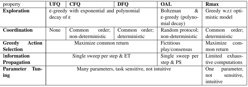
Table 1 summarizes the differences between the three algorithms according to the features men-tioned above.

property UFQ CFQ DFQ OAL Rmax

Exploration ε-greedy with exponential and polynomial

decay ofε

Boltzman &

ε-greedy (polyno-mial decay)

Greedy w.r.t opti-mistic model

Coordination None Common order;

non-deterministic

Common order; deterministic

Random protocol; non-deterministic

Common order; deterministic

Greedy Action

Selection

Maximize common return Fictitious play/consensus

Maximize com-mon return Information

Propagation

Single sweep per step & ET Single sweep per step & PS

Limited exhaus-tive computations

Parameter

Tun-ing

Many parameters, task sensitive, not intuitive One parameter, not sensitive, intuitive

Table 1: Major differences between the experimented algorithms.

3.5 Experimental Results & Analysis

This section describes experiments with the FriendQ, OAL, and Rmax algorithms on three CISGs. The games were designed to evaluate the effects of exploration, coordination, and information-propagation methods on performance in different environments. All games are grid-based. The grid

cells are referred to by (row, column) coordinates indexed from (0,0)at the top left corner of the

(10)

two agents attempt to move into the same cell, they both fail and remain in their current place. Note that in stochastic mode, these rules apply to the actual (stochastic) outcome of the action.

Additionally, for each game, we examined the results of learning by heterogeneous agents, that is, agents using different learning algorithms. Finally, to test how well each algorithm scales up with the number of players, we introduced a fourth game in which the state and action spaces do not grow too fast with the number of players. With this game, we were able to play games with up to 5 players.

Adjusting the parameters of the different algorithms was done by a process of trial and error. The algorithms were repeatedly executed in an experimental setup, varying their parameters between executions until some optimum was reached. The parameters that achieved the best performance were then used throughout. Each set of experimental conditions, other than those related to Rmax,

was subjected to 100 repeated trials. For Rmax, 20 trials were carried out using K1=50, 40 with

K1=100 and 40 with K1=200.8 The discount factor was 0.98 in all trials. Unless mentioned

otherwise, the presented results are averages over all trials. The following parameter settings were tested:

FriendQ

Exploration: ε-greedy with (i) εt ←1/countt0.5000001 where countt is the number of ex-ploratory steps taken by time t. (ii)εt←0.99998countt. (Unless specified otherwise, (i) is used.)9

Learning rate: αs,a←1/n(s,a)0.5000001where n(s,a)is the number of times action a was taken in state s.

Q-value were initialized to 0.

OAL

Exploration: Forε-greedy,εt←1/countt0.5000001, as in FriendQ. For Boltzman exploration,

the temperature parameter was decreased byτ←100/count0.7.

History: Random history sample size k=5. History memory size m=20 (m must satisfy

m≥k×(n+2). OAL withε-greedy exploration is referred to asε-OAL, and OAL with

Boltzman exploration is referred to as B-OAL.

Q-value were initialized to 0.

Rmax

Sampling: values of 50, 100, 200 and 300 for K1 (visits to mark an entry known) were tested.

Accuracy of Policy Iteration: Offline policy iteration was halted when the difference be-tween two successive approximations was less than 0.001.

(11)

3.5.1 GAME1

This game, introduced in Hu and Wellman (1998), was devised to emphasize the effects of equilibrium-selection methods. It has a single goal state (the only reward-yielding state) and several optimal

ways of reaching it. The game is depicted in Figure 1. S(X) and G(X) are the respective initial

and goal positions of agent X . In the goal state G, both agents are in their goal positions and their reward is 48. Upon reaching the goal, the agents are reset to their initial position. The underlying SG has 71 states. The optimal behavior in deterministic mode reaches G in four steps and yields an

average reward per step (a.r.p.s.) of 12.10 There are 11 different optimal equilibria. In stochastic

mode, the optimal policies yield an a.r.p.s. of∼5.285. Algorithms were executed for 107rounds on

both settings.

S(A)

S(B)

G(B)

G(A)

Figure 1: Game 1 - initial and goal states.

Deterministic Mode

Table 2 reports the number of trials (of 100 in total) in which each algorithm learned a policy, with four levels of final performance based on the number of steps required to reach the goal. For this deterministic domain, we find this measure, which is directly correlated with the more standard

a.r.p.s. measure, to be more informative. Here xFQ is a variant of FriendQ in which the agents

explore in unison but do not coordinate exploratory actions. The suffix “εed” denotes exponential

decay ofε. In the present context, the agents’ learning of an optimal policy means that their greedy

choice of actions is optimal. That is, with any residual exploration deactivated. Figure 2 presents the a.r.p.s. obtained by the agents over time.

steps to goal

UFQ CFQ xFQ DFQ DFQεed ε-OAL B-OAL B-OALPS MQ Rmax

4 62 49 47 100 100 26 49 41/60 1 100

5 38 49 46 62 51 19/60 49

6+ 2 7 12 29

∞ 21

Table 2: Game 1 – classification of final performance of learned policies for 100 trials of each algorithm

(12)

0 2 4 6 8 10 12

0 1e+06 2e+06 3e+06 4e+06 5e+06 6e+06 7e+06 8e+06 round number

average reward per step.

FriendQ variants on deterministic Game-1. Average reward over time.

Averaged over 100 trials.

UFQ CFQ xFQ DFQ DFQeed DFQETeed

(a) FriendQ variants

0 2 4 6 8 10 12

0 200000 400000 600000 800000 1e+06 round number

average reward per step.

OAL variants and ModelQ on deterministic Game-1. Average reward over time.

B-OAL e-OAL B-OALPS MQ

(b) OAL variants and MQ

0 2 4 6 8 10 12

0 200000 400000 600000 800000 1e+06 round number

average reward per step

Rmax on deterministic Game-1. Average reward over time. Averaged over 100 trials.

Rmax K1=200 Rmax K1=100 Rmax K1=50 (c) Rmax 0 2 4 6 8 10 12

0 200000 400000 600000 800000 1e+06 round number

Rmax, B-OALPS and DFQETeed on det. Game-1. Average reward over time.

Averaged over 100 trials

DFQETeed Rmax K1=50 B-OALPS

(d) Rmax; OAL; FriendQ

Figure 2: Game 1 – average reward per step under deterministic mode. (a) presents first 8×106

rounds. (b), (c) and (d) present first 106rounds.

(13)

ε-OAL does not present a similar trend. In the trials in which OAL converged to second-best

behavior in the first 2.5×105 rounds, it failed to find an optimal policy even after 107 rounds

(Figure 2b). In DFQ, since exploration is deterministic, this switch is always at the same time,

specifically after 7×106rounds(Fig. 2a).

Surprisingly, UFQ fares better than CFQ (Table 2, Fig. 2a), in spite of its less sophisticated coordination strategy. At an early learning stage, dis-coordination leads to exploration. Later on, the estimated Q-values of optimal actions are rarely equal, and thus, coordinating exploitation does not

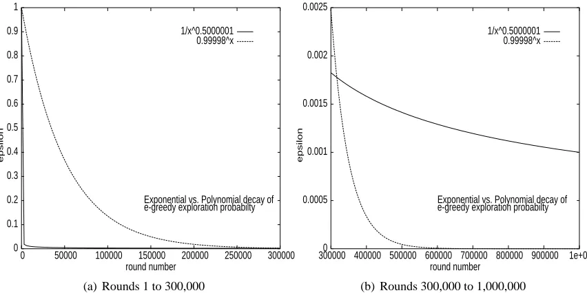
pose a problem (at the examined time interval). Exponential decay ofεsupplies more exploration at

an early period than polynomial decay (Fig. 3) leading to faster convergence of DFQεed (Fig. 2a).

Eligibility traces did not contribute much in this example. The parameters of eligibility traces were hard to tune and very sensitive to change in other parameters or environment dynamics.

0 0.1 0.2 0.3 0.4 0.5 0.6 0.7 0.8 0.9 1

0 50000 100000 150000 200000 250000 300000 round number

epsilon

Exponential vs. Polynomial decay of e-greedy exploration probabilty

1/x^0.5000001 0.99998^x

(a) Rounds 1 to 300,000

0 0.0005 0.001 0.0015 0.002 0.0025

300000 400000 500000 600000 700000 800000 900000 1e+06 round number

epsilon

Exponential vs. Polynomial decay of e-greedy exploration probabilty

1/x^0.5000001 0.99998^x

(b) Rounds 300,000 to 1,000,000

Figure 3: Exponential vs. polynomial decay ofε-greedy exploration probability

OAL agents converge relatively quickly to optimal or second-best behavior, and from that time onwards stick to their behavior (Fig. 2b). Whether, in the latter case, they fail to structure the Q-values properly, or the fictitious play prevents the agents from changing their behavior after the Q-values are ordered properly, is not clear from the data. B-OAL converges faster and more often

to optimal thanε-OAL (Fig. 2b, Table 2). This behavior seems to stem from the effect of the decay

methods we used. The Boltzman method yields more exploration than theε-greedy method in the

early period of learning. Later on,ε-greedy maintains a low exploration probability that decays very

slowly while Boltzman exploration drops faster to zero. Thus, even when ε-OAL learns optimal

behavior, it keeps achieving only near-optimal average-reward.

As expected B-OALPS improves on the performance of B-OAL (Fig. 2b, Table 2) because of its more rapid propagation of learned information.

(14)

early stages of learning, fictitious play amplifies the random behavior. However, at later stages of learning, deviation from constant action choice is rare and will probably not affect fictitious play. In this setting, ModelQ shows slower convergence than the model-free FriendQ.

The learning graph of Rmax can be precisely divided into two periods, an initial learning period in which Rmax attains very low return due to exploration, followed by a period of exploitation in which Rmax attains optimal return (Fig. 2c). The length of the initial period depends linearly on

K1.11 Figure 2d compares the best performing variant of each algorithm.

Stochastic Mode

Figure 4 presents the results for the stochastic mode. As expected, due to the stochastic effects of actions, the value of the optimal policy decreases, and more importantly, the learning algorithms

require more trials to converge. By contrast to the deterministic case, MQ performs as well asε-OAL

(Fig. 4a). This improvement is attributable to additional exploration stemming from the stochastic nature of the environment. For the same reason, CFQ performs almost the same as UFQ (Fig. 4a).

When we compare the gap between the DFQεed to U/CFQ at the first 106rounds in stochastic mode

vs. the deterministic mode we find that the gap is smaller. This difference is due to the fact that the

additional early exploration supplied by the exponential decay of εis redundant in the stochastic

case. The slightly higher return gained by DFQεed later on is due to the faster decay ofε. Another

interesting difference from the deterministic setting is that initiallyε-OAL gains lower return than

B-OAL but while B-OAL keeps attaining the same average reward,ε-OAL improves slowly over

time and eventually gains a higher average reward than B-OAL. In this case, the slower convergence

of the exploration probability to zero enablesε-OAL to “overcome” randomly “bad” exploration in

initial learning phases.

Rmax behaves similarly in stochastic and deterministic modes. While the other algorithms achieve only near-optimal return, Rmax attains optimal return (Fig. 4b,c). Rmax’s strong explo-ration bias results in low return until model entries are known. From that point on, Rmax attains an optimal return. The histogram (Fig. 4d) shows that Rmax converges to higher return than the other algorithms not only in the average case but also in the worst case (i.e., almost all runs of Rmax were better than the best runs for the other algorithms). Very low values for K1, which mean rough transition probability estimates, are enough for computing near-optimal behavior. Indeed, the exploration vs. exploitation tradeoff is evident even in this simple example. We see how a smaller value of K1 leads to faster convergence, but at the cost of slightly smaller average reward.

Overall, it appears that the major issue for the FQ and OAL class of algorithms is exploration. As the space of joint-actions is quite large, there are many relevant options to try. Especially in the deterministic case, the rather standard exploration techniques we used appear to be insufficient. Although stochastic domains naturally lead to more exploration, we can see that the model-free algorithms are sub-optimal. It appears that model-free algorithms—at least in their standard form— have difficulty determining whether certain states were explored sufficiently, and that standard ex-ploration schemes are too crude. Overall, many of the phenomena observed in Game 1 were present in Games 2 and 3. Therefore, in the following experiments, only phenomena not observed in Game 1 will be emphasized.

(15)

1.5 2 2.5 3 3.5 4 4.5 5 5.5

0 1e+06 2e+06 3e+06 4e+06 5e+06 6e+06 7e+06 8e+06 9e+06 1e+07 round number

Variantss of FriendQ and OAL on stochastic Game-1. Average reward over time.

Averaged over 100 trials

UFQ CFQ DFQeed MQ OAL btz OAL eps

(a) FriendQ; OAL; MQ

0 1 2 3 4 5 6

average reward per step in last 10,000 rounds

Rmax on stochastic Game-1. Average reward over time with different K1 values. Averaged over 40 trials, 1,000,000 rounds per trial

Rmax K1=50 Rmax K1=100 Rmax K1=200 Rmax K1=300 (b) Rmax 0 1 2 3 4 5 6

Stochastic Game-1. Average reward over time. Averaged over 100 trials

Rmax K1=100 DFQeed B-OAL

(c) Rmax; FriendQ; OAL

3.8 4 4.2 4.4 4.6 4.8 5 5.2 5.4 5.6 5.8 6

0 20 40 60 80 100

number of experiments

average reward per step of learned policy _{Stochastic Game-1.}

Average reward per step of learned policy against # of trials: x = # of trials in which avg reward of learned policy exceeded y

UFQ CFQ DFQeed Rmax OAL btz OAL eps OAL PS btz

(d) Average reward of learned policies per number of trials

Figure 4: Game 1 – Average reward per step and learned policies per number of trials in stochastic

mode. Subfigures (a) and (c) present all 107 rounds, while (b) presents the first 106

rounds.

3.5.2 GAME2

(16)

moving right(left). However, the object is too heavy for one agent and requires cooperation of the two agents to be moved. The manner by which the object is moved is depicted in Figure 5(b). Note that the push/pull effect is a by-product of the agents’ moves. Thus, in stochastic mode, what determines if the action is push or pull is not the chosen action but its actual effect.

S(A) S(B)

x

G2 G1

(a) Initial state and Goal states.

A ←

B ←

x - x A B

(b1) Moving the object by pushing simultaneously.

(Agents’ order does not matter).

A →

B →

x - A x B

(b2) Moving the object by pushing and pulling simultaneously.

(Agents’ order does not matter).

Figure 5: Game 2

The agents’ goal is to move the object into one of the upper corners of the grid, at which point the game is reset to its initial state. Moving the object to the upper right (G1) or left (G2) corner yields

a reward of 80 and 27, respectively. The optimal behavior under deterministic mode is to move the

object to G1in 8 steps. The average reward per step of an optimal strategy under deterministic mode

is 10, and the discounted return is∼465. The second-best strategy is moving the object to G2in 4

steps, with an a.r.p.s. of 9 and discounted return of∼440. In stochastic mode, the optimal policy

may stochastically lead to one of the goal positions. The a.r.p.s. of the optimal policy in stochastic

mode is ∼3.8. The underlying CISG contains 164 states. Algorithms were executed for 3×107

rounds.

Deterministic Mode

Table 3 classifies the number of trials (of 100 per algorithm) according to the algorithms and learned policies. Figure 6 shows the a.r.p.s. over time obtained by the different algorithms.

The main reasons for the sub-optimal performance of OAL and CFQ in this game are: (i)

Ran-dom exploration has a greater chance of reaching G2 than G1. Discovering G2 before G1 further

reduces the chance of visiting G1 because of the increasing bias toward exploitation. (ii)

Explo-ration of the CFQ and OAL agents is not coordinated. If reaching G2 is the current greedy policy,

then G1 will not be visited unless both agents explore simultaneously. Game 1 demonstrated an

advantage of exponential decay of theε-greedy exploration probability over polynomial decay of

this probability. Game 2 demonstrates an opposite phenomenon, Fig. 6a and Table 3 show that CFQ

does better with polynomial decay ofε than with exponential decay. This result stems from finite

(17)

Goal steps to goal

CFQ CFQεed DFQεed ε-OAL B-OAL Rmax

G1 8 100 1 100

G2 3 99 65 54 91

G2 4 1 35 46 8

Table 3: Game 2 – Characteristics of the learned policy on a per-trial basis for each algorithm in deterministic mode.

7 7.2 7.4 7.6 7.8 8 8.2 8.4 8.6 8.8 9

0 5e+06 1e+07 1.5e+07 2e+07 2.5e+07 3e+07

round number

FriendQ and OAL on deterministic Game-2. Average reward over time.

CFQ CFQeed e-OAL Boltzman OAL

(a) FriendQ and OAL.

0 1 2 3 4 5 6 7 8 9 10

0 500000 1e+06 1.5e+06 2e+06 2.5e+06 3e+06 round number

Rmax, B-OAL and DFQeed on deterministic Game-2. Average reward over time.

Rmax K1=200 Rmax K1=100 Rmax K1=50 B-OAL DFQeed

(b) Rmax; B-OAL; DFQeed.

Figure 6: Game 2 – Average Reward under deterministic mode. Subfigure (a) presents all 3×107

rounds; Subfigure (b) presents first 3×106rounds.

when exploration is coordinated as shown by the learning curve of DFQεed (Fig. 6b) and by Table 3.

Furthermore, DFQεed converges to optimal greedy behavior while both CFQ variants do not.

Stochastic Mode

Figure 7 presents statistics for the stochastic mode. It exhibits two interesting phenomena that have not been observed in the previous experiments. One is that, in contrast to previous results,

ModelQ outperformsε-OAL (Fig. 7a,c). Since the only difference betweenε-OAL and ModelQ is

the greedy action selection method, a reasonable explanation is that BAP (OAL’s action selection mechanism) delays behavioral change that should follow Q-value updates (which in turn may delay learning of Q-values). This outcome is because BAP plays a best response to the strategy implied by the other agent’s past plays. Since both agents react to each other’s past plays using BAP, it may take long to converge to a new NE when the optimal joint actions are changed. The second phenomenon is that Rmax requires larger values of K1 to converge to optimal behavior (Fig. 7b). This finding can be explained by the fact that the optimal behavior involves longer cycles of state transitions and hence the model has to be more accurate.

(18)

Thus, in cooperative multi-agent systems, we face the standard problem, clearly visible in Game 1, of ensuring sufficient exploration, but we need to ensure that this exploration is effective by coordinating exploratory moves of different agents.

1.8 2 2.2 2.4 2.6 2.8 3 3.2 3.4 3.6 3.8

0 5e+06 1e+07 1.5e+07 2e+07 2.5e+07 3e+07

round number

Variantss of FriendQ and OAL stochastic Game-2. Average reward over time.

CFQ DFQ DFQeed MQ B-OAL e-OAL B-OAL PS

(a) FriendQ and OAL

0 0.5 1 1.5 2 2.5 3 3.5 4

0 3e05 6e05 9e05 1.2e+061.5e+061.8e+062.1e+062.4e+062.7e+06 3e+06 round number

Rmax, DFQeed and B-OALPS on stochastic Game-2. Average reward over time.

Averaged over 100 trials (Rmax, averaged over 40 trials). Rmax K1=50 Rmax K1=100 Rmax K1=200 Rmax K1=300 DFQeed B-OAL PS

(b) Rmax; B-OALPS; DFQeed

2 2.2 2.4 2.6 2.8 3 3.2 3.4 3.6 3.8 4

0 20 40 60 80 100

average reward per step of learned policy

number of experiments

Stochastic Game-2.

Histogram of average reward per step of learned policy against number of trials: x = number of trials in which average reward of learned policy exceeded y

CFQ DFQ DFQeed Rmax MQ B-OALPS e-OAL e-OAL

(c) Average Reward of Learned Policies per Number of Trials

Figure 7: Game 2 – Average reward per step and learned policies per number of trials under

stochas-tic mode. (a) presents all 3×107rounds; (b) presents first 3×106rounds.

3.5.3 GAME3

In the previous games, one had to explore considerable parts of the state space in order to construct good policies. This game is characterized by a maximum return attainable by staying in a small

local set of states anywhere on the state graph. The initial position of the agents within a 3×3 grid

is random. They are rewarded for reaching a position in which their locations are adjacent. If this position is attained by unaltered positions of both agents, the reward is 5. If movement is involved,

(19)

As opposed to previous experiments, in deterministic mode, B-OAL and the FriendQ variants converged faster to optimal (greedy) behavior than Rmax (Fig. 8a). Rmax explores the whole model before it starts exploiting while FriendQ’s and OAL’s choice of greedy actions is optimal long before good estimates of all Q-values are attained. However, in stochastic mode the GLIELPs no longer have this advantage since stochastic transitions do not enable the agents to concentrate on exploiting a local set of states (Fig. 8b).

2 3 4 5 6 7 8 9 10

All algorithms on deterministic Game-3. Average reward over time. Averaged over 100 trials

UFQ CFQ MQ e-OAL B-OAL Rmax, K1=200 Rmax K1=100 Rmax K1=50

(a) deterministic mode

0 1 2 3 4 5 6 7 8

All algorithms on stochastic Game-3. Average reward over time.

Each setup except Rmax averaged over 100 trials. Each setup of Rmax averaged over 40 trials.

Rmax K1=50 Rmax K1=100 Rmax K1=200 UFQ CFQ DFQ MQ OAL btz OAL eps

(b) stochastic mode

Figure 8: Game 3 – average reward per step under deterministic and stochastic modes.

3.5.4 HETEROGENEOUSPLAYERS

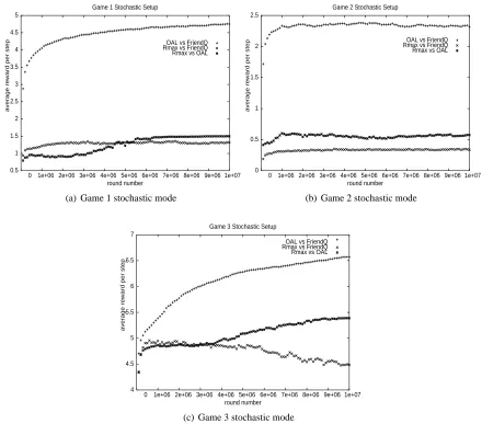
A CISG is most naturally viewed as a model of a distributed stochastic system. As such, it is natural to have in mind a view of a system’s designer, and one would expect such a designer to equip the players with identical algorithms. However, CISGs arise also when self-interested agents need to coordinate, typically on the use of some resource, where coordination is beneficial to all parties involved. Examples include which side of the road to travel on, the meaning attached to a symbol, etc. Thus, it is natural to ask how the algorithms tested fare in the context of other algorithms. We reran the above experiments with pairs of different algorithms. The results, presented in Figure 9 are, quite uniform (similar performance is observed in the deterministic games). The top performance, and as is clearly visible, by a wide margin, was obtained by OAL+FriendQ. Pairs containing Rmax performed much worse, with Rmax+OAL typically fairing slightly better than Rmax+FriendQ. In fact, comparing the results to the homogeneous case, the OAL+FriendQ combination performed almost optimally in Game 1: 4.7 vs. 5. In Game 2 it obtained 2.3 vs. 3.8, and in Game 3 it

achieved 5.85 vs. 7.2.12 And while Rmax and, to a lesser extent, FriendQ do better against their

own kind, OAL does better against FriendQ. It may be the case that for equilibrium selection, OAL’s mechanism works best when one agent ”insists” more on a particular equilibrium, thus more quickly breaking up symmetries.

These results might be interpreted as an indication of the “rigidity” of each of the algorithms. FriendQ is the simplest of the three algorithms, it makes no internal assumptions about its partners

(20)

0.5 1 1.5 2 2.5 3 3.5 4 4.5 5

Game 1 Stochastic Setup

OAL vs FriendQ Rmax vs FriendQ Rmax vs OAL

(a) Game 1 stochastic mode

0 0.5 1 1.5 2 2.5

(b) Game 2 stochastic mode

4 4.5 5 5.5 6 6.5 7

(c) Game 3 stochastic mode

Figure 9: Heterogeneous play games 1-3.

and simply adapts. Rmax is at the other extreme, it strongly relies on the behavior of its partners in order to systematically explore and then exploit. OAL is somewhere in between. It does have a sophisticated mechanism for selecting among different equilibria, but this mechanism is stochastic and can handle noise, and is based on fictitious play, which is a mechanism that adapts to the empirical behavior of the other agents. Thus, one would expect Rmax to fail when its assumptions are not met, as its implicit coordination mechanism is based upon them. In contrast, FriendQ and OAL, which make weak internal assumptions about their peers, should work well, especially when their opponent shows some flexibility and adaptivity.

3.5.5 n>2 PLAYERS

(21)

exponentially with the number of players. Thus, to get an idea of how these algorithms fare with a large number of players, we devised a simpler, fourth game in which we could run experiment with up to 5 players. This is a simple linear grid with 5 positions. Players can move to the left and the right. When two players attempt to move to the same position, the result is with probability 1/3 none move, and with probability 1/3 each one of the players makes the move and the other stays in place. In the initial state, player i is in position 5−i. The goal position of each player is i. Generally, the reward at each state is the number of players located at their goal positions. However, when all players are in their goal position, they receive a reward of 3 times the number of players, at which point all players transition automatically to the initial position.

0 0.5 1 1.5 2 2.5 3 3.5

0 50000 100000 150000 200000 250000 300000 350000 400000 450000 round number

Game 4 Rmax Stochastic Setup

2 Players 3 Players 4 Players 5 Players

(a) Game 4 R-max

0 0.5 1 1.5 2 2.5 3 3.5

0 500000 1000000 1500000 2000000 round number

Game 4 OAL Stochastic Setup

(b) Game 4 OAL

0 0.5 1 1.5 2 2.5 3 3.5

0 500000 1000000 1500000 2000000 round number

Game 4 Friend-Q Stochastic Setup

(c) Game 4 Friend-Q

Figure 10: Results for 2-5 players on game 4.

The results are presented in Figure 10. Note the difference in scale for the X -axis for OAL and FriendQ, which is intended to show that the suboptimal a.r.p.s. to which they converge does not increase even when we look at millions of steps. As in the previous section, we used the CFQ

(22)

For all algorithms, the value is greater as the number of players increases due to the game’s reward definition, which is sensitive to the number of players. All algorithms converge quickly on this game for all number of players. However, the values they converge to differ. Among the three algorithms, Rmax converges to the highest average per step reward, FriendQ is next, and OAL is last. The relative performance is consistent with the performance displayed in the three earlier two-player games. This finding is a reasonable indication that the relative performance of these algorithms is qualitatively similar regardless of the number of players, at least for small player sets.

3.5.6 SUMMARY

Section 3.5 presents an experimental study of three fundamentally different algorithm families for learning in CISGs. The results illustrate the strengths and weaknesses of different aspects of these algorithms in different settings, highlighting the accentuated importance of effective exploration, which is enabled in this class of games only by coordinated behavior, the advantage of deterministic behavior for attaining such coordinated behavior, and the benefits of propagation of information.

Each of the experimental domains emphasizes different aspects of the learning task in CISGs. The results show that the parameters of OAL and FriendQ are very sensitive to environmental topol-ogy and dynamic. Exploration and coordination strategies suitable for one environment may be very inefficient in other environments. Rmax, on the other hand, is stable in this respect. It has a single parameter, K1, that has to be preset. Its convergence time depends linearly on K1 (and the size of the state-action space) and it turns out that Rmax converges to near optimal behavior using values of K1 that achieve faster convergence than that of OAL and FriendQ. However, the convergence dynamics of Rmax does not suit tasks in which the agents must attain some value during the

learn-ing period, because durlearn-ing its exploration phase, Rmax is indifferent to rewards lower than Rmax.

However, Rmax is also the simplest algorithm, and thus it is easy to alter it, for instance, to obtain

satisficing behavior, for example, by lowering the value of Rmaxin the model, or by starting with a

moderate value and then increasing it as better values are observed. Overall, when we control the algorithm of all agents in the system, Rmax seems to be the best alternative—it converges quickly to values higher than those of OAL and FriendQ, it does not seem to be sensitive to an increase in the number of players, except through its effect on the state space, and most importantly, it has very simple exploration strategy. As we saw in games 1 and 2, the choice of exploration strategy has much influence on the results of FriendQ and OAL, and the precise choice is sensitive to the nature of the game, number of equilibria and their nature. Thus, the simple exploration behavior of Rmax and the potential to alter it in various transparent ways is a clear benefit. Yet, when we may need to coordinate with other players with unknown coordination mechanisms, or if our underlying state space is too big for repeated value computations, FriendQ seems to offer the best choice.

4. Learning in FSSGs

In two-player Zero Sum SGs (ZSSGs), the players’ payoffs sum up to zero at every entry. That is,

[R(s,a1_,_a2_)]

1=−[R(s,a1,a2)]2 for every s∈S,a1∈A1 and a2∈A2. Such payoffs indicate that

the agents’ interests completely conflict. A ZSSG can be modeled with a single payoff function R0(s,a1,a2) = [R(s,a1,a2)]1 by redefining Player’s 2 objective as to minimize the IHDR (infinite

horizon discounted reward). For the rest of this section, it is assumed that Player 1 is the

max-imizer and Player 2 is the minmax-imizer the payoff function R. Let V(s,π1,π2) denote the expected

(23)

there-after, and V(π1,π2) = (V(1,π1,π2), ...,V(|S|,π1,π2)). Since the best response in a ZSSG is also the worst for the opponent, ZSSGs have a unique NE value. To see this, assume by negation that V(s,π1,π2)>V(s,µ1,µ2)and that both(π1,π2)and(µ1,µ2)are NE. Sinceπ2∈BR(π1), it follows

that V(s,π1,µ2)≥V(s,π1,π2)>V(s,µ1,µ2), which contradicts µ1∈BR(µ2). The value of a policy

πmay be defined as V(π,BR(π)). In ZSSGs, this definition coincides with that of a NE (any pair of

optimal policies is a NE and vice versa).

Consequently, the state-value function V(s)is redefined to be the expected IHDR under a profile

of optimal policies and Q(s,a1,a2)the expected IHDR for taking joint action(a1,a2)in state s and

continuing according to a NE thereafter. For any stationary strategy profile(π1,π2) in a ZSSG G,

(π1(s),π2(s))is a NE for the matrix games defined by[Q(s,a1,a2)]_a1_∈_A

1,a2∈A2 for all s∈S if and

only if(π1,π2)is a NE for G and the NE values for the matrix games correspond to the state values

V(s,π1,π2)(Filar and Vrieze, 1997). Thus, the Bellman optimality equations can be rewritten for

ZSSGs as

Q∗(s,a1,a2) = R(s,a1,a2) +γ

∑

s0

T(s,a1,a2,s0)V∗(s0)

V∗(s) =

∑

a1_∈_A

1,a2∈A2

π1(a1)π2(a2)Q(s,a1,a2) (1)

where(π1,π2)is a NE for the matrix game defined by the Q-values in state s. Given a method that

computes NE for zero sum matrix games, Equation (1) can be used as an iterative approximation rule to compute the Q-values (Littman, 1994) and given the Q-values an optimal policy can be derived. The NE policies for a zero sum matrix game M= [r(ai,bj)]ik=,l1,j=1are the solutions to the

linear program that maximizes v under the constraints (Filar and Vrieze, 1997)

(

k

∑

i=1

π(ai)r(ai,bj)≥v|j∈ {1, ...,l}

)

.

In the following sections, this linear program is abbreviated as:

v= max

π∈PD(A)minb∈B_a

∑

_∈_Aπ(a)r(a,b).

If SG G is obtained from ZSSG G0by adding a constant c to all payoffs of both players, then

V_iG(π1,π2) =V_iG0(π1,π2) +c/(1−γ)for any policy profile(π1,π2) and the strategic properties of the game are unchanged. G is referred to as a Fixed Sum Stochastic Game (FSSG). The adversarial nature of FSSGs calls for agents that perform well not only in self play but also in heterogeneous play, namely when engaged by agents that employ different learning algorithms. Under this setting, the exploration/exploitation tradeoff wears a new guise as attempted exploration and exploitation may be interfered by the opponent.

(24)

4.1 FoeQ

FoeQ (a.k.a MinimaxQ) (Littman, 1994, 2001) extends Q-learning into FSSGs by using a sample

backup learning rule based on Equation 1 (Littman, 1994). After taking a joint action(a,b)in state

s at time t and reaching state s0 with reward rcur, the agent updates the Q-value ofhs,(a,b)iby

Qt(s,a,b)←(1−αt)Qt−1(s,a,b) +αt rcur+γ max

π∈PD(A)minb0_∈_B

∑

a0_∈_A

π(a0)Q(s0,a0,b0)

!

.

Qtconverges in the limit to Q∗under the standard Q-learning conditions stated in Section 3.1. Also,

for similar reasons to those stated in Section 3.1, FoeQ is executed with anε-greedy learning policy.

4.2 WoLF

WoLF (Bowling and Veloso, 2002) is designed to converge to a best response rather than a NE. WoLF does not explicitly consider an adversary. It applies the standard single-agent Q-learning rule to approximate Q-values of private actions and uses hill climbing to update its mixed policy. That is, the policy is improved by increasing the probability of selecting a greedy action according to a

policy learning rateδ(which is distinct from the Q-value learning rateα), enabling mixed policies.

The uniqueness of WoLF is in using a variable policy learning rate according to the “Win or Learn Fast” (hence WoLF) principle: if the expected return of the current policy given the current Q-values

is below (above) a certain threshold then a high,δl (low,δw), learning rate is set. A good threshold

would be the NE value of the game because if the player is receiving less than its value, its likely playing a sub-optimal strategy, whereas if it receives more than the NE value, the other players must be playing sub-optimally. Since the NE value is unknown, it is approximated by the expected return of the average policy (averaged over the history of the game) given the current Q-values. The motivation for the WoLF variable policy learning rate is to enable convergence to a NE. Indeed, Bowling and Veloso (2002) show that gradient ascent with WoLF is guaranteed to converge to a NE in self play on two-player, two-action, repeated matrix-games, while gradient ascent without a variable learning rate is shown not to. Furthermore, they provide empirical results on FSSGs in which WoLF converges to NE in self play. WoLF, as single agent Q-learning, is guaranteed to converge in the limit to a best response under the standard conditions and given that the opponent(s) converge to stationary policies.

4.3 Rmax

Section 3.3 describes the Rmax algorithm in the context of MDPs. The same algorithm is applicable to FSSGs with the only difference that joint actions are considered and optimal policies with respect to the fictitious model are computed according to (1). As mentioned in Section 3.3, Rmax always

behaves optimally with respect to an approximated, initially optimistic, model M0of the real model