R E S E A R C H
Open Access
Spatial-temporal analysis of non-Hodgkin
lymphoma in the NCI-SEER NHL case-control study
David C Wheeler
1*, Anneclaire J De Roos
2, James R Cerhan
3, Lindsay M Morton
4, Richard Severson
5,
Wendy Cozen
6and Mary H Ward
1Abstract
Background:Exploring spatial-temporal patterns of disease incidence through cluster analysis identifies areas of significantly elevated or decreased risk, providing potential clues about disease risk factors. Little is known about the etiology of non-Hodgkin lymphoma (NHL), or the latency period that might be relevant for environmental exposures, and there are no published spatial-temporal cluster studies of NHL.
Methods:We conducted a population-based case-control study of NHL in four National Cancer Institute (NCI)-Surveillance, Epidemiology, and End Results (SEER) centers: Detroit, Iowa, Los Angeles, and Seattle during 1998-2000. Using 20-year residential histories, we used generalized additive models adjusted for known risk factors to model spatially the probability that an individual had NHL and to identify clusters of elevated or decreased NHL risk. We evaluated models at five different time periods to explore the presence of clusters in a time frame of etiologic relevance.
Results:The best model fit was for residential locations 20 years prior to diagnosis in Detroit, Iowa, and Los Angeles. We found statistically significant areas of elevated risk of NHL in three of the four study areas (Detroit, Iowa, and Los Angeles) at a lag time of 20 years. The two areas of significantly elevated risk in the Los Angeles study area were detected only at a time lag of 20 years. Clusters in Detroit and Iowa were detected at several time points.
Conclusions:We found significant spatial clusters of NHL after allowing for disease latency and residential mobility. Our results show the importance of evaluating residential histories when studying spatial patterns of cancer.
Background
From 1975 to 2000 in the United States, the annual age-adjusted incidence rate of non-Hodgkin lymphoma (NHL) increased more than 75% from 11.1 to 19.8 per 100,000 person-years [1]. The incidence rate has leveled recently, to 19.6 per 100,000 person-years between 2003-2007 [2]. An increase in incidence also occurred in other developed countries; for example, incidence increased across Europe since the 1960s [3]. The cause of the increases is largely undetermined and little is known in general about the etiology of NHL.
Incidence of NHL increases with age, is 40-70% higher in whites compared to blacks, and is higher in men [4].
Established risk factors include specific viruses, immune suppression, and a family history of hematolymphoproli-ferative cancers [5]. Other putative risk factors include specific genetic polymorphisms [6-8], certain occupa-tions [9], and environmental exposures such as pesti-cides [10], polychlorinated biphenyls (PCBs) [11,12], and organic solvents [13]. Previous studies have found higher risk of NHL among persons living in areas with indus-trial waste exposure [14-17]. Associations with these risk factors are generally moderate-to-weak in strength or inconsistent in the literature. Taken together, the established and putative risk factors account only for a small proportion of the total annual NHL cases [5]. In addition, little is known about the latency period that might be relevant for environmental exposures. Novel approaches are needed to generate insights into the etiology of NHL.
Investigating spatial-temporal patterns of disease inci-dence through cluster detection analysis identifies areas * Correspondence: [email protected]
1
Occupational and Environmental Epidemiology Branch, Division of Cancer Epidemiology and Genetics, National Cancer Institute (NCI), National Institutes of Health (NIH), Department of Health and Human Services (DHHS), Bethesda, MD, USA
Full list of author information is available at the end of the article
with significantly different disease risks than the overall population under study. A cluster is typically considered to be an area of significantly elevated disease risk, but it could also be an area of significantly lowered risk. We note the distinction in goals between detecting local clusters and approaches to describe global clustering of disease, the general tendency for cases to occur nearer other cases than one might expect under equal risk [18-20]. The identification of local clusters can lead to the development of specific hypotheses to explain the pattern of risk and reveal important clues about disease etiology [21].
However, limitations in existing methods for evaluating clusters in space and time in epidemiologic studies have hindered cluster analyses. No previous cluster analyses of NHL has adjusted for individual-level risk factors and modeled disease latency in one unified statistical frame-work. Existing cluster detection techniques as applied to case-control or cohort studies [22-24] do not allow for simple adjustment of confounding variables using all data simultaneously in the cluster detection model. Typically, either a pre-processing regression analysis must be done before the cluster analysis to adjust for risk factors or several cluster analyses must be performed on strata of the data, where stratified analyses will be limited by small sample sizes. In a cluster analysis, the residential loca-tions of study subjects at time of diagnosis are typically considered a surrogate for environmental exposures defined broadly to include lifestyle factors such as diet, in addition to pollutants, and spatially-varying socioeco-nomic factors. Using the diagnosis location makes the unrealistic assumption that individuals do not migrate and that the latency between causal exposures and diag-nosis of disease is negligible [25]. Cluster studies that make use of residential history data in epidemiologic stu-dies typically assume one latency period with little empirical justification. Some studies have included all historical residential locations for each subject in one sta-tistical model with an assumption of independent obser-vations, which can bias model results by ignoring many correlated records in the model for each subject [26-28].
To date, there have been no published spatial-temporal cluster studies of NHL using residential history data. We evaluated residential histories for NHL cases and controls in the National Cancer Institute (NCI) Surveillance, Epi-demiology, and End Results (SEER) NHL (NCI-SEER NHL) case-control study to determine if there were sta-tistically significant spatial clusters of NHL using several time windows of residential location. The NCI-SEER NHL study is a large, multi-center, population-based case-control study of NHL in four areas of the United States (Detroit, Los Angeles, Seattle, Iowa). We devel-oped a statistical approach for cluster analysis based on the established generalized additive model (GAM)
framework. We extended previous work [26-29] applying GAMs to model spatial variability in disease risk by con-sidering the temporal aspect of disease risk as a model selection problem in a GAM. We hypothesized that after adjusting for NHL risk factors there would be significant spatial clusters of NHL cases due to unmeasured envir-onmental risk factors, and that earlier residential loca-tions, up to 20 years before diagnosis, would model NHL risk better than residence at diagnosis.
Methods
Study population
The study population, described in detail previously [5,6,30], included 1,321 NHL cases diagnosed between July 1, 1998 and June 30, 2000, aged 20 to 74 years, from four SEER registries. The four SEER areas were: Macomb, Oakland, and Wayne counties for Detroit; Los Angeles County; King and Snohomish counties for Seattle, and the state of Iowa. Self-reported HIV-positive cases were excluded from the study. Population controls (n = 1,057) were selected from residents of the four SEER areas using random digit dialing (< 65 years) or Medicare eligibility files (≥65 years), frequency matching to cases by age (within 5-year groups), sex, race, and SEER area. Controls with a history of NHL or known HIV infection were excluded. Among eligible subjects contacted for an inter-view, 76% of cases and 52% of controls participated in the study.
Interviews were conducted in 1998 to 2000. A computer-assisted personal interview was administered that con-tained questions about various potential risk factors for NHL, including occupation, home and garden use of pesti-cides, diet, hair dyes, alcohol and tobacco, and viruses [5,6,30]. All participants were sent a lifetime residential calendar in advance of the in-person interview. They were asked to provide their complete address for every home they lived in from birth to the current year, indicating the year they moved in and out by a vertical line between each home; they were also asked to provide information about temporary or summer homes where they lived for a total of two years or longer. Interviewers reviewed the residential calendar with respondents and probed to obtain missing information.
We excluded residences that were address matched to the level of a populated place, county centroid, or state centroid. In addition to exact matches, we included resi-dences matched to intersections (8.8% of addresses) or ZIP Code centroids (5% of addresses). Most of the addresses matched to the ZIP Code level were located in Iowa; there was no obvious spatial pattern in these addresses. To maintain a consistent dataset while explor-ing the effect of different residence location time periods on the risk of NHL, we included participants who had a 20-year history of continuous residential location within one of the four SEER centers. The percent of addresses that were matched to a populated place or state or county centroid (excluded in analysis) generally increased with increasing time before enrollment, requiring a bal-ance between potentially long latencies of interest and data quality. For each participant, we included all resi-dential locations within 2 miles of each study area boundary. A total of 842 cases (64%) and 680 controls (64%) met our criteria for inclusion in this analysis. Sum-mary statistics for the frequency-matching variables are listed in Table 1. The cases and controls were distributed fairly evenly across the four study centers. Residential mobility was similar across the study areas. The median number and quartiles (lower, upper) of addresses per subject in each study center were 2 (1, 2) in Detroit, Iowa, and Seattle, and 1 (1, 3) in Los Angeles.
Statistical models
We used generalized additive models [31,32] to model spatially the probability that an individual had NHL within each SEER center study area. GAMs have been used to model the probability of disease in other case-control cluster analyses [26-28]. Our GAM-based approach is different from previous approaches in how we modeled multiple residence periods, treating selec-tion of the optimal residential time period as a model selection problem. The optimal time period can be con-sidered as the time in years before diagnosis of NHL or reference date (controls) when etiologically-relevant exposure(s) occurred and we hereafter refer to it as the lag time. We fitted crude models and models adjusted for several factors associated with NHL in our study population and available for all cases and controls in our analysis, including age, gender, race, education, and home treatment for termites before 1988 as a surrogate for exposure to the pesticide chlordane. Other NHL risk factors for this study population, such as PCB levels in the current home and levels of PCBs and furans in the blood, were available for only a subset of the subjects and were omitted in this analysis to maximize the num-ber of subjects studied.
We considered a binary response variable Yfor NHL case status with associatedP(Y= 1) =p(s,x) depending
on the explanatory variablesxand the spatial locations, which consists of the coordinates (s1,s2). Given the
resi-dential locationsstfor subjects at a particular time t, the log odds of being a case is modeled as
logit[pi(x,s)] =α+ Xiβ+Zt(st), (1)
where the left-hand side of the equation is the log of the disease odds for subjecti,a is an intercept, b is a column vector of regression coefficients, Xi is a row of the matrix of covariates, andZt(st) is a smooth function of the residential locations at a particular time t. The GAM framework is flexible, as the model in equation (1) becomes a crude spatial model when no covariates are specified, a logistic regression model when no spatial smoothing term is specified, and the null model when neither covariates nor a spatial smoothing term are spe-cified (intercept only). Adjusting for known risk factors may explain a cluster observed in a crude analysis or may identify clusters not seen in a crude analysis. Any spatial cluster observed after adjustment for known risk factors would be the subject of further study to identify unknown spatially varying risk factors.
The functionZt(s) is a spatial smoothing of the loca-tions and models spatial variation not explained by the covariates. The spatially smoothed term may be consid-ered a surrogate for unmeasured environmental expo-sures at a specified time. The smoothing function is used as a measure of the density of cases relative to controls over space. This approach models cases and controls as a marked heterogeneous Poisson point process with inten-sityl(s) =l1(s) +l0(s), wherel1(s) is the intensity of
cases andl0(s) is the intensity of controls. The related
technique of kernel intensity estimation [33,34] uses the ratio of the intensities of point processes for controls and cases to yield a spatial odds function, but because of its limitation to easily adjust for covariates, we selected the GAM framework.
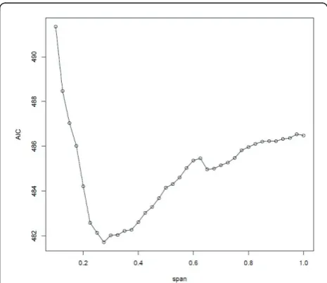
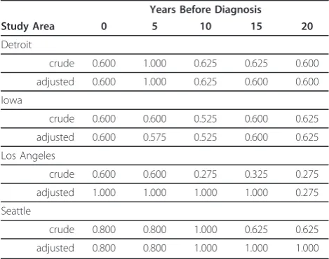
the difference between the local minimum AIC and the global minimum AIC was not meaningful. We used the previously suggested guideline of 3 as a meaningful dif-ference in AIC [38,39]. The approach of using smaller spans with local minimum AIC to emphasize local varia-tion in risk has been used previously [27,28]. As an exam-ple of span selection, the selected span of 0.275 in the crude model for the Los Angeles center at a residential time lag of 20 years had the globally minimizing AIC (Figure 1). The spans selected for all latency periods for each study area are listed in Table 2. As a sensitivity ana-lysis, we also repeated the analysis with the global span if it was different from the chosen span.
We estimated the GAM model parameters in the statis-tical analysis software R [40] using the gam package, which is written by Trevor Hastie and is an implementa-tion of the GAM framework of Hastie and Tibshirani [31]. While there are other options available for smooth-ing spline functions in gam and in the R package mgcv, we chose loess because its span parameter is the most readily interpreted.
Mapping risk
To produce a map of local odds ratios (ORs) of NHL from the GAM model, we first estimated all parameters for the model expressed in equation (1) using the study
data. We then predicted the log odds over a rectangular grid over the study area using the estimated model para-meters. We used a 50 × 50 grid (2,500 cells) based on the minimum and maximum coordinates of each study Table 1 Descriptive statistics for analysis population and NCI-SEER NHL study population
Cases (n = 842) Controls (n = 680) Analysis Total (n = 1522) Study Total (n = 2378)
Study Center, %
Detroit 25 21 24 22
Iowa 32 31 31 27
Los Angeles 23 24 23 25
Seattle 20 24 22 26
Age, mean years
Detroit 57 61 59 56
Iowa 61 63 62 59
Los Angeles 60 60 60 56
Seattle 60 61 61 57
Males, %
Detroit 53 45 50 52
Iowa 50 52 51 51
Los Angeles 55 52 54 55
Seattle 49 51 50 53
White, %
Detroit 82 75 79 76
Iowa 98 99 99 98
Los Angeles 77 61 70 66
Seattle 94 93 93 90
Note: Analysis population excluded subjects address matched to the level of a populated place, county centroid, or state centroid and/or who did not live in the study area for 20 years.
area. We assigned covariate values to the grid for adjusted models. To provide an interpretable odds ratio map, we used the analysis population for each SEER center as the reference and divided the odds from the spatial model at each grid point by the odds from the null model. This approach has been used previously [28] and yields a local odds ratio that is interpretable in rela-tion to the overall study area. For example, an OR of 1.8 at a specific location means that the rate of NHL there is elevated 80% compared with the entire study area.
To evaluate the local odds ratios for statistical signifi-cance in crude and adjusted models, we used pointwise permutation distributions. This type of assessment is com-mon practice in kernel density estimation [18,34] and has also been used in other GAM-based approaches [26-28]. Informally, to identify areas of significantly elevated dis-ease risk, or clusters, we determine if the observed elevated odds ratios are more extreme than we would expect under the null hypothesis that case status does not depend on location. Pointwise permutation distributions are built through iterative Monte Carlo randomization of case sta-tus to compare the observed local odds ratio at a location to the distribution of local odds ratios under the null hypothesis at that location [18]. The Monte Carlo rando-mization first conditions on the residential locations and then randomizes the case labels among the fixed locations. For each randomization of the case labels, the spatial model parameters are estimated and then used to predict the local odds ratios on the grid. This procedure is repeated 999 times to build a distribution of local odds ratios at each location on the grid. We identified areas of significantly elevated risk as those areas that had an observed odds ratio in the upper 2.5% of the ranked per-mutation distribution of odds ratios. Similarly, we identi-fied areas of significantly lowered risk of NHL as those
having an observed odds ratio in the lower 2.5% of the ranked permutation distribution. Clusters of elevated risk are identified with contours of the 97.5 percentile of the pointwise permutation distributions of local odds ratios, therefore they are significant at the 0.05 level (assuming a two-tailed distribution).
It is noteworthy that the Monte Carlo randomization technique for evaluating significance provides pointwise statistical inference, not overall inference due to the multiple locations of evaluation and the correlation in local odds ratios from the sharing of data in the smoothing function at nearby locations [19]. As a result, this method should be used to identify clusters of signif-icantly elevated and decreased risk, but not to identify the most likely cluster in the study area.
Evaluation of residential lag time
To determine which residential location time period was most associated with NHL risk, we included in models for each center the smoothed spatial pattern of subject resi-dences at the time of diagnosis and also at four time peri-ods before diagnosis. We chose 5, 10, 15, and 20 years for both the crude and adjusted models. We tested the effect of different lag times on NHL risk through analysis of deviance (ANODEV), testing for significant differences between model deviances from the model with no smoothing term and from the five models with smoothing terms (one for time at diagnosis, four with lag times). Spe-cifically, we estimated equation (1) for time at diagnosis (Z0) and for each lag time of interest (Zk) and statistically
tested the deviances from the models with aZterm and the deviance from the model with noZterm. The differ-ence in deviances for two nested models approximately follows a chi-square distribution with an associated p-value. The p-value for each ANODEV test indicates the probability of achieving a reduction in deviance equal to the difference in model deviances for a number of degrees of freedom equal to the difference of model degrees of freedom when using one model nested in another model. These p-values should be interpreted with caution, as recent work has shown that chi-square p-values for smoothed terms in GAMs tend to have inflated type I error rates [41]. A significantly lower deviance from a model with a lag time ofkyears means that using the smoothed pattern of residential locations fromkyears ago significantly explains overall NHL risk. The lag-time model with the smallest p-value from analysis of deviance best explains the risk of NHL. The test of the term for smoothed residential locations tests for an overall spatial pattern in NHL risk, and as such may be considered as a type of global test of spatial variation of disease. This glo-bal test evaluates a different property of the disease pattern than the Monte Carlo randomization process described earlier, which tests for local clusters of elevated NHL risk. Table 2 Smoothing span values for the crude and
adjusted models for the SEER study areas
Years Before Diagnosis
Study Area 0 5 10 15 20
Detroit
crude 0.600 1.000 0.625 0.625 0.600
adjusted 0.600 1.000 0.625 0.600 0.600
Iowa
crude 0.600 0.600 0.525 0.600 0.625
adjusted 0.600 0.575 0.525 0.600 0.625
Los Angeles
crude 0.600 0.600 0.275 0.325 0.275
adjusted 1.000 1.000 1.000 1.000 0.275
Seattle
crude 0.800 0.800 1.000 0.625 0.625
Evaluation of potential selection bias
Because response rates were relatively low for both cases and controls, we investigated the possibility that selec-tion bias affected the results of our spatial cluster analy-sis. The concern was that clusters detected in study participants could be due to differential participation among cases and controls. For example, a high density of nonparticipating controls and low density of nonpar-ticipating cases in an area could produce an artificial cluster of elevated risk. To explore this possibility, we performed additional cluster analyses among study parti-cipants and nonpartiparti-cipants in each center using the GAM approach described above, but limited to a single time point.
Current addresses and demographics (age, race, gen-der) were available for all eligible cases (from the registry) and for controls 65 and older (from Centers for Medicare & Medicaid Services). Eligibility of younger controls was determined by a telephone survey in which gender, age, and the residential address were obtained. We first per-formed a spatial cluster analysis for participants only with crude models and models adjusted for only age and gender. We then performed a cluster analysis for partici-pants and nonparticipartici-pants together. We were primarily interested in clusters of elevated risk in participants that were not present in the analysis with participants and nonparticipants.
Because nonresponse to the telephone survey resulted in incomplete ascertainment of eligible controls less than 65 years of age, we also performed a separate eva-luation of nonresponse bias restricted to participants aged 65 years or more.
Results
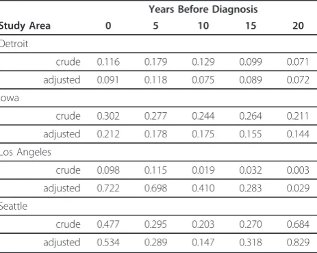
In our analysis of residential locations at several time per-iods, the most significant lag time was 20 years according to both crude and adjusted models (Table 3) in three centers: Detroit (crude and adjusted models p-value = 0.07), Iowa (crude model p-value = 0.21, adjusted model p-value = 0.14), and Los Angeles (crude model p-value = 0.003, adjusted model p-value = 0.03). In Seattle, the most significant lag time was 10 years for both the crude (p-value = 0.20) and the adjusted (p-value = 0.15) models. Overall, the results showed that a residential lag time of 20 years best explained risk of NHL associated with spa-tially-dependent exposures in our study.
Among the adjusted models, only the lag time of 20 years for Los Angeles was statistically significant at the 0.05 level. The lag time of 20 years for Detroit was mar-ginally statistically significant (p-value=0.07). It is worth noting that the p-value for a lag time of 20 years for Los Angeles was an order of magnitude lower than for other lag times in this study center. Such a marked difference among lag times was not found in the other study
centers. It is also noteworthy that whereas p-values for the analysis of deviance of crude models in Los Angeles for the lag times of 10, 15, and 20 years were statistically significant at the 0.05 level, after adjusting for known risk factors the contribution of the residual spatial term to the log odds of NHL was no longer statistically signif-icant for lag times of 10 and 15 years.
Using the most significant lag time identified in crude and adjusted models, we found significant clusters of ele-vated NHL risk in three of the study centers (Detroit, Iowa, and Los Angeles). In the Detroit center, there was an area of elevated risk in southeast Oakland County near the junction of Oakland, Macomb, and Wayne counties at a lag time of 20 years (Figure 2). In addition to the area of significantly elevated risk, we also found a cluster of rela-tively low risk of NHL in northwestern Wayne County. The presence and general location of clusters were consis-tent between the crude and adjusted models; however, there were differences in the shapes of the clusters. In Detroit, the cluster detected by the adjusted model is lar-ger and has a greater risk of NHL than does the cluster in the same area detected by the crude model.
There was a statistically significant cluster of elevated risk in south-central Iowa at a lag time of 20 years that included most of Wayne, and parts of Appanoose, Davis, and Lucas counties in the adjusted model (Figure 3). There were no clusters of lowered risk. There were two significant areas of elevated risk in the Los Angeles study area at a 20-year lag time (Figure 4). One cluster was located in northwestern Los Angeles County, with cases located in the large geographic but sparsely populated northwestern part of Los Angeles County. A small cluster of elevated risk was also found in the city of Los Angeles, in West Hollywood. This cluster appeared as a high risk area for NHL, corresponding to an area with a high Table 3 Analysis of deviance test p-values for crude and adjusted models in the SEER study areas
Years Before Diagnosis
Study Area 0 5 10 15 20
Detroit
crude 0.116 0.179 0.129 0.099 0.071
adjusted 0.091 0.118 0.075 0.089 0.072
Iowa
crude 0.302 0.277 0.244 0.264 0.211
adjusted 0.212 0.178 0.175 0.155 0.144
Los Angeles
crude 0.098 0.115 0.019 0.032 0.003
adjusted 0.722 0.698 0.410 0.283 0.029
Seattle
crude 0.477 0.295 0.203 0.270 0.684
prevalence of HIV positive individuals in an earlier study conducted at the census tract level [42]. There was also a small cluster of lowered risk detected in mostly Hispanic southeast Los Angeles County. We found no statistically significant clusters in the Seattle center at the 10-year lag
time in either the crude or adjusted models (Figure 5). Our sensitivity analysis of selected span values revealed that the patterns of local odds ratios were smoother with the larger spans, but the locations of clusters generally remained the same (data not shown).
Figure 2Crude and adjusted local odds ratios (OR, scale at right) for NHL at a residential lag time of 20 years in the Detroit study area. Clusters of statistically significant elevated odds ratios are identified with a solid white line and statistically significant lowered odds ratios are identified with a dashed black line. Crude model: span = 0.6 (p-value = 0.07); Adjusted model: span = 0.6 (p-value = 0.07). Model adjusted for age, gender, race, education, and home termite treatment before 1988.
Figure 4Crude and adjusted local odds ratios (OR, scale at right) for NHL at a residential lag time of 20 years in the Los Angeles study area. Clusters of statistically significant elevated odds ratios are identified with a solid white line and statistically significant lowered ORs are identified with a dashed black line. Crude model: span = 0.275 (p-value = 0.003); Adjusted model: span = 0.275 (p-value = 0.03). Model adjusted for age, gender, race, education, and home termite treatment before 1988.
While our primary approach was to evaluate spatial clusters at the lag time most strongly associated with risk of NHL, we also plotted the local odds ratios and signifi-cant contour lines at the other time periods to determine if the local clusters were detected at multiple time lags. We used the optimal span for each lag time. In Detroit, the area of elevated risk was present at the time of diag-nosis and at 5 and 15 years before diagdiag-nosis, in addition to 20 years. The area of elevated risk in Iowa was detected at all five time periods. In contrast, the clusters of elevated and decreased risk in Los Angeles were found only at the 20-year lag time (Figure 6). No clusters were found in Seattle at any time periods.
The results from the cluster analyses for all partici-pants versus all eligible cases and controls were gener-ally similar for each study area. For example, the pattern of elevated risk in Detroit at time of diagnosis for all eli-gible cases and controls was similar to that for partici-pants, although the location of statistically significant clusters shifted somewhat (Figure 7). The cluster of
lowered risk in Wayne County was not observed when including all eligible cases and controls. However, the area of significant elevated risk found in participants of the study is not fully explained by selection bias, as much of the cluster in southern Oakland County remains after including nonparticipants in the analysis. The results from the cluster analyses for participants aged 65 or more and eligible cases and controls aged 65 years or more were also similar across the study areas. For example, the overall pattern of risk of NHL in Los Angeles at time of diagnosis is similar with no areas of statistically significant risk (Figure 8).
Discussion
Our approach to modeling spatial variation in disease risk extends earlier work with generalized additive mod-els by evaluating several residential time windows as a model selection problem using residential histories in a case-control study. The spatial analysis of NHL risk in the NCI-SEER NHL study provided evidence that
residential location at 20 years, the longest lag time we evaluated, explained NHL risk better than residence location at times closer to diagnosis. We found that there were areas of statistically significant risk of NHL in several of the study areas. Detroit and Iowa each had a cluster of elevated risk after adjusting for known indi-vidual-level risk factors. The cluster in Iowa was found in five residential time periods and the cluster in Detroit was found in four time periods. The Los Angeles study area had two clusters that were present only at a lag time of 20 years. The Seattle study area had no clusters. Despite the presence of local clusters, there was not consistent evidence across the study areas for significant overall spatial variation in NHL risk. It is possible to have local clusters without an overall pattern of cluster-ing [18,19,43,44]. Our results demonstrate the impor-tance of considering past residential locations in a cluster analysis. Here, we elaborate on some features of our analysis, including the evaluation of various lag times, adjustment for risk factors, and some specific considerations of the modeling approach.
To our knowledge, this is the first spatial cluster analyses of a case-control study of NHL using residential histories to account for residential mobility. Cluster studies often use the residence location at time of diagnosis, thereby assuming the relevant environmental exposure or risk fac-tor occurred at the diagnosis address. This will be true for some subjects, but certainly not for others. Previous clus-ter studies [26-28] using generalized additive models included in one model all possible residences for each sub-ject before a lag time of interest, resulting in a biased model with several correlated records per subject. With such an approach, a detected cluster could be the result of a few cases moving around within a small area over time [27]. A previous study restricted one analysis to the resi-dence of longest duration and found somewhat different results in cancer cluster locations than when using multi-ple addresses per subject with a latency of 20 years [27]. Previous studies have also assumed certain lag times with-out quantitative justification of the particular choice. In contrast, we treated the selection of the lag time as a model selection problem, where the smoothed functions of the residences at specific lag times are treated as model terms; the term that best explains disease risk suggests the most relevant lag time. While our modeling approach allows for testing the significance of different time periods, the model assumes one relevant residential lag time, i.e. one location for exposure. It is possible, however, that exposures occur at more than one residential location. In other words, exposure could be cumulative over time and space. To consider this, in future work we will develop methods to include several residential locations for each person in one model. Such an approach is a step toward
encompassing life-course environmental exposures, the idea of the“exposome”[45].
In our study, we adjusted for several potential confound-ing variables in a spatial cluster model. Often cluster stu-dies do not adjust for known risk factors, aside from basic demographics. Any covariate that has a spatial pattern and is associated with the outcome could cause confounding of the association of the outcome and unmeasured envir-onmental exposure, as represented by the smoothed func-tion of residential locafunc-tions. After adjustment for confounders, an observed cluster may become nonsignifi-cant. Conversely, adjusting for known risk factors can also identify hidden clusters in a crude analysis. Other cluster detection techniques, such as the local scanning method in SaTScan [22,23] and Q-statistics [24], do not allow for adjustment of confounding variables in a case-control or cohort study in a unified statistical cluster-analysis model. In our study, adjusting for known risk factors made certain clusters more prominent and revealed a pattern of increased risk for NHL in Detroit and Iowa. A cluster in Los Angeles decreased in size with adjustment. While we adjusted for several risk factors, our adjustment did not include all possible risk factors of NHL. In future work, we will explore the observed clusters for the presence of sig-nificant variables in other datasets, such as the U.S. Cen-sus, Environmental Protection Agency (EPA) Toxic Release Inventory, and the Census of Manufacturers and the Census of Agriculture.
There are several aspects of the generalized additive model framework to consider when performing cluster analysis, including the span selection and possible edge effects. Span selection is important because patterns in the local odds ratio maps derived from GAMs depend on the span. A small span will reveal more local variation in risk, while a larger span will produce a smoother pattern of risk. Using an automatic search routine to select the span with the smallest Akaike information criterion may lead to selecting a span with a local minimum AIC and not a global minimum. To avoid this, we selected the span visually from a graph of AIC values for a range of spans. However, this approach can suggest several span values with local minima that are very close in AIC to the global minimum. We favored smaller values of the span when the difference in AIC for a local minimum and a global minimum was not meaningful to identify impor-tant features of the disease point process. Sensitivity ana-lysis with larger spans did not change the presence and locations of observed clusters.
function for smoothing over residential locations. Loess uses a tri-cube weight function that gives less weight to data points farther from the estimation point [31,35,36]. Due to this weighting function, loess should exhibit smal-ler edge effects than an alternative smoother based on nearest neighbors with equal weights [28]. In a previous simulation study, Webster et al. [28] found little evidence of edge effects interfering with estimating the true odds ratio surface using loess as the spatial smoother in a gen-eralized additive model. We also sought to minimize edge effects to some degree by including residential loca-tions within 2 miles of each study area boundary.
In general, results of a cluster analysis should be inter-preted carefully due to potential selection bias. Response rates were relatively low for both cases and controls in the NCI-SEER NHL study. Differences in the distributions of respondents and nonrespondents may make case and con-trol groups unrepresentative of the base population in terms of exposure prevalence. However, the risk estimate will only be biased if a risk factor differentially influences participation among controls and cases [46]. Previously, we analyzed spatial patterns in nonresponse separately by study center and by case status using a spatial scan statistic [30]. Two significant elliptical clusters in Detroit and Los Angeles were nonsignificant after adjusting for demo-graphic factors. We also found that the nonresponse bias in NHL risk associated with education level was not large. De Roos et al. [47] found evidence of selection bias in the NCI-SEER study when investigating proximity to indus-trial facilities and risk of NHL. Current residences of parti-cipants were less likely to be located within 2 miles of an industrial facility than were those of nonparticipants. The differences in proximity to industry by participation were accounted for by variation in select census block group-level demographic variables. Although proportions of par-ticipants and nonparpar-ticipants living within 2 miles of an industrial facility were significantly different, the associa-tion between proximity of current residence to one or more industry and NHL risk did not differ by participa-tion. In our comparative cluster analyses of participants and all eligible cases and controls at time of study enroll-ment, we did not find substantial differences in patterns of elevated risk. Clusters of elevated risk in participants were not explained by including nonparticipants in the analysis. The results suggested that the response bias was not responsible for the clusters of elevated risk detected among study participants. Our assessment of bias, how-ever, was limited to only residences at time of selection into the study.
Conclusions
After adjusting for several known risk factors, we found evidence of several clusters of elevated NHL risk in the NCI-SEER NHL study. We also found that long lag
times of residential location were more likely than shorter lag times to result in significant clusters of ele-vated NHL risk in several study areas. Results of this study will lead to future investigations to evaluate possi-ble reasons for the significant clusters, which may lead to new hypotheses about the etiology of NHL. We per-formed our cluster analyses using generalized additive models, which provide a unified statistical framework for estimating disease risk spatially and assessing signifi-cance of elevated risk for case-control and cohort data. It is straightforward to adjust for covariates and evaluate several temporal lags in this statistical framework. This study serves as an illustrative example for those inter-ested in performing space-time cluster analysis of dis-eases without well-known etiologies and this approach can be useful in the generation of new hypotheses.
List of Abbreviations
OR: Odds Ratio; NHL: Non-Hodgkin Lymphoma; EPA: Environmental Protection Agency; ANODEV: Analysis of Deviance; AIC: Akaike Information Criterion; PCB: Polychlorinated Biphenyl; NCI: National Cancer Institute; SEER: Surveillance, Epidemiology, and End Results; GAM: Generalized Additive Model
Acknowledgements
We gratefully acknowledge Lonn Irish (Information Management Services, Inc., Silver Spring, MD) for assistance in data processing and preparation and Thomas M. Mack, MD, MPH (University of Southern California) for comments on a draft of the manuscript. This study was supported by the National Cancer Institute’s Surveillance, Epidemiology and End Results Program under contracts PC-35139, N01 PC065064, NO1-PC-67008, PC-71105, N01-PC67009, P01 CA17054, P30 ES07048, P30 CA014089, and the Centers for Disease Control and Prevention’s National Program of Cancer Registries, under agreement #U55/CCR921930-02.
Author details 1
Occupational and Environmental Epidemiology Branch, Division of Cancer Epidemiology and Genetics, National Cancer Institute (NCI), National Institutes of Health (NIH), Department of Health and Human Services (DHHS), Bethesda, MD, USA.2Fred Hutchinson Cancer Research Center and University
of Washington, Seattle, WA.3Mayo Clinic College of Medicine, Rochester,
MN, USA.4Radiation Epidemiology Branch, Division of Cancer Epidemiology
and Genetics, NCI, NIH, DHHS, Bethesda, MD, USA.5Department of Family
Medicine and Karmanos Cancer Institute, Wayne State University, Detroit, MI, USA.6Department of Preventive Medicine and Pathology, and Norris
Comprehensive Cancer Center, USC Keck School of Medicine, University of Southern California, Los Angeles, CA, USA.
Authors’contributions
DW conceived of the study, performed the statistical analysis, and drafted the manuscript. MW participated in the design of the study and helped to draft the manuscript. ADR, JC, RS, WC, and LM participated in the design and conduct of the case-control study. All authors read and approved the final manuscript.
Competing interests
The authors declare that they have no competing interests.
Received: 19 April 2011 Accepted: 30 June 2011 Published: 30 June 2011
References
2. Altekruse S, Kosary C, Krapcho M, Neyman N, Aminou R, Waldron W, Ruhl J, Howlader N, Tatalovich Z, Cho H, Mariotto A, Eisner M, Lewis D, Cronin K, Chen H, Feuer E, Stinchcomb D, Edwards B:SEER Cancer Statistics Review.
Bethesda, MD: National Cancer Institute; 1975.
3. Parkin D, Bray F, Ferlay J, Pisani P:Global cancer statistics.CA Cancer J Clin
2002,55:74-108.
4. Jemal A, Tiwari R, Murray T, Ghafoor A, Samuels A, Ward E, Feuer E, Thun M:
Cancer Statistics.CA Cancer J Clin2004,54.
5. Chatterjee N, Hartge P, Cerhan J, Cozen W, Davis S, Ishibe N, Colt J, Goldin L, Severson R:Risk of non-Hodgkin’s lymphoma and family history of lymphatic, hematologic, and other cancers.Cancer Epidemiol Biomarkers Prev2004,13:1415-1421.
6. Morton L, Wang S, Cozen W, Linet M, Chatterjee N, Davis S, Severson R, Colt J, Vasef M, Rothman N, Blair A, Bernstein L, Cross A, De Roos A, Engels E, Hein D, Hill D, Kelemen L, Lim U, Lynch C, Schenk M, Wacholder S, Ward M, Zahm S, Chanock S, Cerhan J, Hartge P:Etiologic heterogeneity among non-Hodgkin lymphoma subtypes.Blood2008,112:5150-5160. 7. Skibola C, Bracci P, Nieters A, Brooks-Wilson A, de Sanjosé S, Hughes A,
Cerhan J, DR S, Purdue M, Kane E, Lan Q, Foretova L, Schenk M, Spinelli J, Slager S, De Roos A, Smith M, Roman E, Cozen W, Boffetta P, Kricker A, Zheng T, Lightfoot T, Cocco P, Benavente Y, Zhang Y, Hartge P, Linet M, Becker N, Brennan P,et al:Tumor necrosis factor (TNF) and lymphotoxin-alpha (LTA) polymorphisms and risk of non-Hodgkin lymphoma in the InterLymph Consortium.Am J Epidemiol2010,171:267-276.
8. Skibola C, Curry J, Nieters A:Genetic susceptibility to lymphoma. Haematologica2007,92:960-969.
9. Khuder S, Schaub E, Keller-Byrne J:Meta-analyses of non-Hodgkin lymphoma and farming.Scand J Work Environ Health1998,24:255-261. 10. Zahm S, Weisenburger D, Babbitt P, Saal R, Vaught J, Cantor K, Blair A:A case-control study of non-Hodgkin’s lymphoma and the herbicide 2,4-dicholorophenoxyacetic acids (2,4-D) in eastern Nebraska.Epidemiology
1990,1:349-356.
11. De Roos A, Hartge P, Lubin J, Colt J, Davis S, Cerhan J, Severson R, Cozen W, Patterson DJ, Needham L, Rothman N:Persistent organochlorine chemicals in plasma and risk of non-Hodgkin’s lymphoma.Cancer Res2005,
65:11214-11226.
12. Colt J, Severson R, Lubin J, Rothman N, Camann D, Davis S, Cerhan J, Cozen W, Hartge P:Organochlorines in carpet dust and non-Hodgkin lymphoma.Epidemiology2005,16:516-525.
13. Fritschi L, Benke G, Hughes A, Kricker A, Turner J, Vajdic C, Grulich A, Milliken S, Kaldor J, Armstrong B:Occupational exposure to pesticides and risk of non-Hodgkin’s lymphoma.Am J Epidemiol2005,162:849-857. 14. Goldberg M, Siemiatyck J, DeWar R, Desy M, Riberdy H:Risk of developing
cancer relative to living near a municipal solid waste landfill site in Montreal, Quebec, Canada.Arch Environ Health1999,54:291-296. 15. Dreiher J, Novack V, Barachana M, Yerushalmi R, Lugassy G, Shpilberg O:
Non-Hodgkin’s lympohma and residential proximity to toxic industrial waste in southern Israel.Haematologica2005,90:1709-1710.
16. Floret N, Frederic M, Bruno C, Arveux P, Cahn J, Viel J:Dioxin emissions from a solid waste incinerator and risk of non-Hodgkin lymphoma.Epidemiology
2003,14:392-398.
17. Bithell J, Dutton S, Draper G, Neary N:Distribution of childhood leukaemias and non-Hodgkin’s lymphomas near nuclear installations in England and Wales.BMJ1994,309.
18. Waller L, Gotway C:Applied Spatial Statistics for Public Health DataNew York: John Wiley; 2004.
19. Waller L:Detection of clustering in spatial data.InThe SAGE Handbook of Spatial Analysis.Edited by: Fotheringham A, Rogerson P. Sage Publications Ltd; 2009:.
20. Besag J, Newell J:The detection of clusters in rare diseases.Journal of the Royal Statistical Society, Series A1991,154:143-155.
21. Blot W, Fraumeni J Jr, Mason T, Hoover R:Developing clues to environmental cancer: a stepwise approach with the use of cancer mortality data.Environmental Health Perspectives1979,32:53-58. 22. Kulldorff M:SaTScan: software for the spatial and space-time scan
statistics.Silver Spring, MD: Information Management Services Inc; 2006. 23. Kulldorff M:A spatial scan statistic.Communications in Statistics: Theory and
Methods1997,26:1487-1496.
24. Jacquez G, Kaufmann A, Meliker J, Goovaerts P, AvRuskin G, Nriagu J:
Global, local and focused geographic clustering for case-control data with residential histories.Environmental Health2005,4.
25. Jacquez G:Current practices in the spatial analysis of cancer: flies in the ointment.International Journal of Health Geographics2004,3.
26. Vieira V, Webster T, Weinberg J, Aschengrau A:Spatial analysis of bladder, kidney, and pancreatic cancer on upper Cape Cod: an application of generalized additive models to case-control data.Environmental Health
2009,8.
27. Vieira V, Webster T, Weinberg J, Aschengrau A, Ozonoff D:Spatial analysis of lung, colorectal, and breast cancer on Cape Cod: an application of generalized additive models to case-control data.Environmental Health
2005,4.
28. Webster T, Vieira V, Weinberg J, Aschengrau A:Method for mapping population-based case-controls studies: an application using generalized additive models.International Journal of Health Geographics2006,5.
29. Kelsall J, Diggle P:Spatial variation in risk of disease: a nonparametric binary regression approach.Applied Statistics1998,47:559-573. 30. Shen M, Cozen W, Huang L, Colt J, De Roos A, Severson R, Cerhan J,
Bernstein L, Morton L, Pickle L, Ward M:Census and geographic differences between respondents and nonrespondents in a case-control study of non-Hodgkin lymphoma.American Journal of Epidemiology2008,
167:350-361.
31. Hastie T, Tibshirani R:Generalized Additive ModelsLondon: Chapman & Hall; 1990.
32. Wood S:Generalized Additive Models: An Introduction with RBoca Raton: Chapman & Hall/CRC; 2006.
33. Kelsall J, Diggle P:Kernel estimation of relative risk.Bernoulli1995,1:3-16. 34. Kelsall J, Diggle P:Non-parametric estimation of spatial variation in
relative risk.Statistics in Medicine1995,14:2335-2342.
35. Cleveland W:Robust locally weighted regression and smoothing scatterplots.Journal of the American Statistical Association1979,74:829-836. 36. Cleveland W, Devlin S:Locally-weighted regression: an approach to
regression analysis by local fitting.Journal of the American Statistical Association1988,83:596-610.
37. Akaike H:Information theory and an extension of the maximum likelihood principle.InInternational Symposium on Information Theory.
Edited by: Petran B, Csaaki F. Budapest, Hungary; 1973:267-281. 38. Burnham K, Anderson D:Model Selection and Multimodel Inference: A
Practical Information-theoretic Approach.2 edition. New York: Springer-Verlag; 2002.
39. Spiegelhalter D, Best N, Carlin B, van der Linde A:Bayesian measures of model complexity and fit.Journal of the Royal Statistical Society, Series B
2002,64:583-639.
40. R Development Core Team: Vienna, Austria: R Foundation for Statistical Computing; 2010, R: A Language and Environment for Statistical Computing.
41. Young R, Weinberg J, Vieira V, Ozonoff A, Webster T:Generalized additive models and inflated type I error rates of smoother significance tests. Computational Statistics and Data Analysis2011,55:366-374.
42. Mack T:Cancers in the Urban Environment: Patterns of Malignant Disease in Los Angeles County and its NeighborhoodsSan Diego, CA: Elsevier Academic Press; 2004.
43. Waller L, Hill E, Rudd R:The geography of power: statistical performance of tests of clusters and clustering in heterogeneous populations. Statistics in Medicine2006,25:853-865.
44. Wheeler D:A comparison of spatial clustering and cluster detection techniques for childhood leukemia incidence in Ohio, 1996 - 2003. International Journal of Health Geographics2007,6.
45. Wild C:Complementing the genome with an“exposome": the outstanding challenge of environmental exposure measurement in molecular epidemiology.Cancer Epidemiol Biomarkers Prev2005,
14:1847-1850.
46. Austin M, Criqui M, Barrett-Connor E, Holdbrook M:The effect of response bias on the odds ratio.Am J Epidemiol1981,114:137-143.
47. De Roos A, Hartge P, Colt J, Blair A, Airola M, Severson R, Cozen W, Cerhan J, Davis S, Nuckols J, Ward M:Residential proximity to industrial facilities and risk of non-Hodgkin lymphoma.Environ Res2010,110:70-78.
doi:10.1186/1476-069X-10-63
Cite this article as:Wheeleret al.:Spatial-temporal analysis of
non-Hodgkin lymphoma in the NCI-SEER NHL case-control study.Environmental