R E S E A R C H A R T I C L E
Open Access
A comparison of time dependent Cox
regression, pooled logistic regression and
cross sectional pooling with simulations
and an application to the Framingham
Heart Study
Julius S. Ngwa
1,2*, Howard J. Cabral
1, Debbie M. Cheng
1, Michael J. Pencina
3, David R. Gagnon
1,
Michael P. LaValley
1and L. Adrienne Cupples
1,4*Abstract
Background:Typical survival studies follow individuals to an event and measure explanatory variables for that event, sometimes repeatedly over the course of follow up. The Cox regression model has been used widely in the analyses of time to diagnosis or death from disease. The associations between the survival outcome and time dependent measures may be biased unless they are modeled appropriately.
Methods:In this paper we explore the Time Dependent Cox Regression Model (TDCM), which quantifies the effect of repeated measures of covariates in the analysis of time to event data. This model is commonly used in
biomedical research but sometimes does not explicitly adjust for the times at which time dependent explanatory variables are measured. This approach can yield different estimates of association compared to a model that adjusts for these times. In order to address the question of how different these estimates are from a statistical perspective, we compare the TDCM to Pooled Logistic Regression (PLR) and Cross Sectional Pooling (CSP), considering models that adjust and do not adjust for time in PLR and CSP.
Results:In a series of simulations we found that time adjusted CSP provided identical results to the TDCM while the PLR showed larger parameter estimates compared to the time adjusted CSP and the TDCM in scenarios with high event rates. We also observed upwardly biased estimates in the unadjusted CSP and unadjusted PLR methods. The time adjusted PLR had a positive bias in the time dependent Age effect with reduced bias when the event rate is low. The PLR methods showed a negative bias in the Sex effect, a subject level covariate, when compared to the other methods. The Cox models yielded reliable estimates for the Sex effect in all scenarios considered.
Conclusions:We conclude that survival analyses that explicitly account in the statistical model for the times at which time dependent covariates are measured provide more reliable estimates compared to unadjusted analyses. We present results from the Framingham Heart Study in which lipid measurements and myocardial infarction data events were collected over a period of 26 years.
Keywords:Time dependent covariate model (TDCM), Cross sectional pooling (CSP), Pooled logistic regression (PLR), Longitudinal and survival data
* Correspondence:[email protected];[email protected]
1Department of Biostatistics, Boston University, School of Public Health, 801
Massachusetts Ave, CT 3rd Floor, Boston, MA 02118, USA Full list of author information is available at the end of the article
Background
A time dependent explanatory variable is one whose value for a subject may change over the period of time that the subject is observed [1, 2]. The most common type of time dependent covariate is a repeated measure-ment on a subject or perhaps a change in the subject’s treatment. Data for a subject can be presented as mul-tiple observations, each of which applies to a time inter-val of observation, which is usually the time period between the exams when the longitudinal measures were recorded. The Cox proportional hazard regression model is often used to analyze covariate information that changes over time, with the hazard proportional to the instantaneous probability of an event at a particular time [3, 4]. Typical settings where time dependent covariates occur include HIV studies in which baseline characteris-tics are recorded and immunological measures such as CD4+ lymphocyte counts or viral load are measured re-peatedly to assess patients’ health until HIV conversion. Therneau and Grambsch considered a well-known ex-ample of the time dependent Cox model (TDCM) using the Stanford Heart Transplant Program [3].
There is extensive literature and a wide range of statis-tical packages for modeling time dependent covariate data. Some previous work includes Fisher and Lin [1]; Cupples et al. [5]; D’Agostino et al. [6]; Pepe and Cai [7]; Prentice and Gloeckler [8]; Abbott [9]; Green and Symons [10]; Ingram and Kleinman [11]; Kalbfleisch and Prentice [12]; Wu and Ware [13].
Models that can accommodate time-dependent covari-ates are commonly used in biomedical research but sometimes do not explicitly adjust for time in the model. Not adjusting for time can yield different estimates of association compared to a model that adjusts for time. In order to address the question of how different these estimates are, we compare three methods that model the association between a longitudinal process and a time-to-event outcome. We consider the TDCM in which the longitudinal measures are used as time dependent covar-iates in a Cox model [4]. We compare the TDCM to Pooled Logistic Regression (PLR) and Cross Sectional Pooling (CSP). The PLR and CSP methods pool observa-tions over disjoint time intervals of equal length into a single sample in order to predict the short term risk of the event. The CSP, unlike the PLR, utilizes information on the length of time to event in each interval as well as whether or not the event occurs. We consider models that adjust and do not adjust for the timing of the longi-tudinal measures in the PLR and also time-interval and non-time-interval models for the CSP. In this paper we refer to all CSP stratified models with time intervals as time adjusted models.
The Framingham Heart Study (FHS) has been collecting data prospectively since 1948 to examine the relationship
of potential risk factors to the development of cardiovas-cular disease [5]. Since risk factors for disease have been collected prospectively and repeatedly measured over time (every 2–4 years), the FHS provides an important example to study various approaches for survival analysis with re-peated measures. The PLR has been frequently employed in the analysis of FHS data [5, 6]. For FHS, the PLR treats the two to four-year examination interval as a mini-follow up study in which the current risk factors are updated at the interval start to predict events during the interval. In this paper we applied the above methods to FHS data in which triglycerides (TG) were measured at generally com-parable time intervals, about every 4 years, over a 26-year period in the FHS Offspring cohort. Time to myocardial infarction was also recorded for each participant, with some subjects remaining free of myocardial infarction at the end of the study period and these subjects were administratively censored at that time. The research protocols of the Framingham Heart Study are reviewed annually by the Institutional Review Board of the Boston University Medical Center and by the Observational Studies Monitoring Board of the National Heart, Lung and Blood Institute. Participants signed a consent form approved by the Institutional Review Board.
Our main objectives are to: (i) compare the TDCM to Pooled Logistic Regression (time adjusted and un-adjusted models) and Cross Sectional Pooling (time ad-justed and unadad-justed models) in simulation studies; and (ii) illustrate the methods and compare their results by applying them to FHS data. We begin by presenting an overview of these methods for modeling time dependent covariates in the context of longitudinal and survival data. We then evaluate the methods using simulation studies and conclude with a discussion of the results from the simulation and the Framingham Heart Study.
Methods
In modeling longitudinal and survival data the main focus may be on the longitudinal component, the survival com-ponent, or both, depending on the objectives of a study. When the focus is on one aspect, the other component is then secondary; so its parameters may be viewed as nuisance parameters [14]. Our goal is to characterize the relation between time-to-event (dependent) and the longitudinal measures (independent) in models that ac-count for the time at which the longitudinal measures are recorded.
In this section, we consider methods for modeling the association between longitudinal measures and time-to-event data in a survival model. We consider the under-lying model to include longitudinal response data and time-to-event data for a sample of size n, consisting of [Ti
*
Yi(t) = [Yi1(t),…,Yip(t)]tis a set of longitudinal measures,
and mi≤p is the number of time intervals for the i th
subject. In addition, each subject has possibly right cen-sored failure Ti= min(Ti* , Ci) and the event indicator δi (δi= 1 if Ti*≤Ci; δi= 0 if Ti* >Ci). The parameter δi
indicates whether the observed failure time is a true fail-ure timeTi*, or a censoring timeCi.
The study design that we consider in our paper has fixed time points where each person has observations at which covariates are measured. Such a study design is common for longitudinal studies. In particular, individ-uals are measured for a time-varying covariate (Y) at the beginning of each time interval and all intervals are of the same length (in our simulations, 5 years). In this context, the regression coefficients represent the associ-ation between Y and an event that occurs during the subsequent interval. We require this study design in order to compare the PLR model, which does not explicitly con-sider time, with those approaches that do incorporate time into the model. For CSP and TDCM, time intervals of equal length are not needed as an assumption of the model. In all the models that we considered, the assump-tion is that the time dependent covariates remain constant between examination times.
Time dependent Cox regression modeling
A time dependent explanatory variable is one that may change over the period of time that the subject is ob-served [2]. The most common time dependent covari-ates are repeated measures on a subject or a change in the subject’s treatment. A proportional hazard model is often used to analyze covariate information that changes over time. One way of handling time-dependent re-peated measurements in SAS is to specify programming statements to capture the appropriate covariate values of the subjects in each time interval of observation. TDCM can be fit using the standard partial likelihood for the Cox model where the values for the time dependent co-variates are updated in each of the event-specific likeli-hood terms.
The hazard for the TDCM at timetcan be written as:
h tð; Yi; XiÞ ¼h0ð Þ t exp Yið Þt Tβþ XiTα
¼h0ð Þ t exp Xmi
k¼1
Yikð Þt Tβkþ XiTα !
ð1Þ
Where h0(t) represents the baseline hazard function, Xi is a vector of time invariant explanatory covariates
with regression parameters. Yik(t) is a general covariate
form in whichmi=pis the number of longitudinal
mea-sures for each subjecti. We definet1<t2<t3<…<tDas
a set of ordered observed event times with D unique
failure times and Yi(ti) as the covariates associated with
the individual whose failure time istifori= 1,…,D
fail-ure times. The parameter βk measures the association between the observed longitudinal measures and the hazard of failure time h(t). The risk set R(ti) at failure
time ti is the set of all individuals who are still under
study at a time just prior toti. In most applications,βk= 0
for intervals other than the current one (ti). The partial
likelihood based on the hazard function specified in (1) can be written as:
Lðα; βÞ ¼Y D
i¼1
exp Yið Þti Tβþ XiTα
X
lR tð Þi exp Ylð Þti
Tβþ XlTα
h i
8 < :
9 = ;
ð2Þ
In the partial likelihood above, each term is the condi-tional probability of choosing individual i to fail from the risk set, given the risk set at failure timetiand given
that one failure occurs. The inference is similar to the Cox model. The only difference is that the values of
Yi(ti) now change for each risk set. The α and β
esti-mates can be obtained by maximizing the likelihood in (2). In TDCM the covariates are measured repeatedly and an assumption of this model is that the hazard de-pends on the covariate through its current value.
Pooled repeated observations
The use of standard logistic regression techniques to es-timate hazard rates was detailed by Efron [15]. His ap-proach, known as partial logistic regression, entailed the use of parametric logistic regression modeling on cen-sored data to obtain estimates and standard errors. The pooled repeated observations approach, described by Cupples et al. [5], has been frequently employed in the Framingham Heart Study. In this method each observa-tion interval is considered a mini-follow up study in which the current risk factors are updated to predict events in the interval. Once an individual has an event in a particular interval all subsequent intervals from that individual are excluded from the analysis.
Pooled logistic regression (PLR)
Ln P tðk;Yi; XiÞ 1−P tðk;Yi; XiÞ
¼βo þYið Þtk TγþXiTαþθk
ð3Þ
The parameter βo is the intercept for the logistic model. The Yi(tk) represent the observed longitudinal
measures for the interval; the parameter θkdenotes the effect of time tk. The time point tk is an element of the
vector representing when the longitudinal measures were recorded. Thus, this model adjusts for the interval in which the observations were made. In our application of this model, we assumed a linear trend on the time ef-fects θk. One drawback of PLR is that the model does not utilize information for the point in time during the interval at which an event occurs or the exact time in an interval that an individual is lost to follow-up. Thus, the contribution of the risk factor to disease is dependent on the length of follow-up period [10]. While there may be concern with the PLR regarding the dependence of mul-tiple records within an individual contributing to several intervals, Allison (2010) has noted that in working with a dataset with multiple records for intervals within each individual there is no inflation of test statistics resulting from a lack of independence [16]. This property is due to the fact that the likelihood factors into a distinct term for each interval. Allison also cautioned that this conclu-sion may not apply when the dataset includes multiple events for each individual. Singer and Willett (2003) also noted that the hazard, or odds in PLR, describes the conditional probability of event occurrence, where the conditioning depends upon the individual survival until that particular time period. This allows all records within the person-period dataset to be considered as condition-ally independent [17].
We should also note that the PLR model provides esti-mates of conditional odds ratios for having the event in an interval rather than of the hazard ratio. Efron [15] discussed the use of the logistic model for survival data and showed that this approach gives direct estimates of the hazard rate and provides approximate standard er-rors. They refer to this parametric model as partial logis-tic regressions due to its connection to Cox’s (1975, ex. 2) theory of partial likelihood. Moreover, Efron’s condi-tional logistic regression model and pooled logistic
regression are equivalent when the length of time inter-val tends towards zero. Green and Symons [10] found that when the follow-up period is short and the event is rare, the logistic regression estimates and their standard errors approximate those from the proportional hazards mode.
Cross sectional pooling (CSP)
The CSP uses Cox regression within interval to utilize information on the length of time to event within each interval as well as whether or not the event occurs. The model relates the instantaneous risk of an event to the longitudinal measures though a hazard function.
hjðt;Yi; XiÞ ¼hj0ð Þ t exp Yið Þt TγþXiTα
ð4Þ
Where hj0(t) represents the baseline hazard function
for the jth interval, γ is the association parameter; t is the time-to-event in the interval. In the time adjusted CSP a stratified Cox model is implemented with time in-tervals (j) when longitudinal measurements were taken. In the unadjusted model, the hazard is assumed to be the same across all time intervals and analysis is per-formed without stratification. In stratified Cox with time intervals, the regression coefficients are assumed to be the same in each interval; however, the baseline hazard function may vary.
Simulation studies
We conducted a series of simulations to evaluate the performance of the CSP, TDCM and PLR methods for modeling longitudinal and survival data. We structured the simulated data to resemble observed data from the Framingham Heart Study as the covariates were mea-sured at specific time intervals (each ~4 years) and held fixed until the next measurement time point. For the simulations we used 5 year intervals. In Table 1, we pro-vide the simulation model and the parameters used for simulating the longitudinal and survival data. The longi-tudinal trajectories were generated from a linear model with age of the participant at entry into the study as a predictor, while survival times were generated using a Weibull model to depend on the longitudinal measures and an additional set of covariates, possibly time-varying.
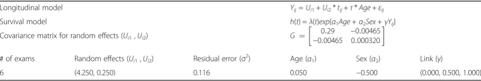
Table 1Model and parameters in simulation study
Longitudinal model Yij=Ui1+Ui2*tij+τ*Age+εij
Survival model h(t) =λ(t)exp{α1Age+α2Sex+γYij}
Covariance matrix for random effects (Ui1,Ui2) G ¼ 0:29 −0:00465 −0:00465 0:000320
# of exams Random effects (Ui1,Ui2) Residual error (σ2) Age (α1) Sex (α2) Link (γ)
6 (4.250, 0.250) 0.116 0.050 −0.500 (0.000, 0.500, 1.000)
In each 5-year time period if the survival time was less than or equal to the time period of the mini follow-up de-fined by the timing of longitudinal measures, then the event was considered to be observed and the time-to-event in that interval was the survival time; otherwise the time-to-event for the interval was censored at the end of the interval [18]. We assumed random non-informative right censoring for subjects remaining event free through the last time interval. We present an algorithm below for generating the simulated data.
We simulated independent multivariate datasets con-sisting of longitudinal measures and time-to-event out-comes. The following algorithm was implemented to generate the longitudinal data using steps 1–5 and the survival data using steps 6 and 7:
Longitudinal component
1. Generate baseline covariates similar to FHS. a. Baseline Age ~normal(35,5) and Sex ~Bernoulli
(0.54)
2. Generate longitudinal trajectories (φβ(tij)) for each
subject (i= 1, 2,…,n) and for each time point (j= 1, 2,…,mi) using the linear model: φβ(tij) =Ui1+Ui2*tij+τ*Age
a. Parameter estimates for the mean and variance-covariance matrix (G) of the random effects, covariance matrix and residual errors were obtained by fitting a random effects model to the FHS data.
b. Generate random effects (Ui1,Ui2) from a
bivariate normal distribution with mean and variance-covariance (G) obtained (2a). The random effects (Ui1,Ui2) represent the intercept and slope.
3. Generate the observed longitudinal measures (Y) from a multivariate normal distribution with mean
φβ(tij) and variance (V):V ¼ZiGZiT þRi; where
Zi¼
1 0
1 5
1 10
1 15
1 20
1 25
2 6 6 6 6 6 6 4
3 7 7 7 7 7 7 5
and Riediagmatrixð Þσ2
In our simulation models the continuously changing values of the triglycerides (covariates) are measured at regular 5 year intervals. The models are designed to cap-ture the covariate measurements at specific longitudinal time points similar to the Framingham Heart Study.
Survival Component:
4. Choose parameter estimate values for Age, Sex and the link parameter which measures the strength of the association between the longitudinal measures and the time-to-event.
5. Generate the time-to-event (T) for each time period in which the longitudinal measures were taken, from the inverse of the cumulative hazard distribution. Survival times generated with the Cox proportional hazard model using the Exponential and Weibull distributions. When the shape is equal to 1, the Weibull distribution equals the exponential distribution. By varying the shape parameter and the scale parameter, the required event rates (10 %, 50 %, and 90 %) can be attained for the survival data.
h(t;Age,Sex,Yij) =λ(t)exp{α1Age+α2Sex+γYij}.
Survival times are generated for each interval to de-pend on the longitudinal measures at the beginning of the interval and a set of covariates (Age at each exam and Sex). The survival time for each participant was computed by considering the cumulative survival time across intervals until an event occurred. Subjects with-out an event at the last interval are censored after the 5-year period of the interval.
The parameter estimates used in our simulations for the random effects, covariance matrix and residual er-rors were obtained by fitting a random effects model to the FHS Data. Baseline age at entry to the study was simulated from a normal distribution with mean 35 and standard deviation 5; sex was assigned according to a draw from a Bernoulli distribution with proportion fe-male = 0.54; these parameters are similar to those of the FHS Data. The observed longitudinal measures (Yij) were
generated from a multivariate normal distribution with means and variances specified above in the simulation scheme. Survival time was generated for each interval using the value of age from the start of the interval. The survival time for each participant was computed by con-sidering the cumulative survival time across intervals until an event occurred. Each replicated data set was simulated to contain 1000 subjects with up to 6 observa-tion intervals. We fit the methods described in secobserva-tion 2 to analyze each of 1000 replicated data sets and used 10,000 replicates to evaluate Type I error. We assessed the performance of these methods using bias, accuracy and coverage. Bias was assessed as the deviation in the estimate from the true simulated parameter. Mean square error (MSE) provided a measure of overall accur-acy by incorporating the bias and the variability. Cover-age of the confidence interval was the proportion of times the obtained confidence interval contains the true specified value.
Pooled logistic regression (PLR_AD). In Table 2 we provide a comparison of the similarities and differences across the different methods. In the CSP and PLR methods Age at each exam was included in the model as a time varying co-variate; the data structure had multiple rows per subject where each row was considered a mini-follow up study in which the current risk factors were updated to predict events in the interval. In the TDCM the baseline Age vari-able was included in the model; the data structure was a single row per subject where the overall survival time was specified for each subject for analysis in SAS. We also ran a model in which a time dependent Age was implemented for the TDCM and we obtained the same results. For CSP and PLR the Age at each exam was calculated by adding the difference in time from the current exam and the first exam to the Age at baseline. In the analysis with these methods, updating age did not make a difference as any update occurred by the same amount for everyone. In the time adjusted PLR, we adjusted for the time inter-val in which the longitudinal measures were recorded by including a time variable (coded as 0, 5, 10, 15, 20 and 25) in the model. In the time adjusted CSP we used a stratified Cox with time intervals to adjust for the different time intervals in which the longitudinal measures were recorded. The statistical analyses were performed using SAS Software (version 9.3; SAS Institute, Cary, NC) and data simulation was performed in R (R Development Core Team, 2012).
Results
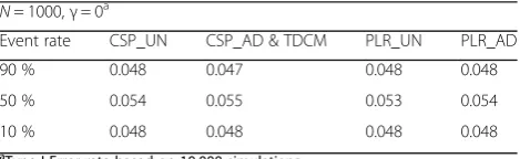
We present results from the simulation studies for the methods described in section 2. Type I errors were com-puted for the longitudinal effect on survival, (γ= 0), using 10,000 replicates and a sample size of 1000 (Table 3). In all simulation schemes the time adjusted CSP (CSP_AD) and TDCM provided identical results, as expected. The time adjusted and the unadjusted methods pro-vided Type I error rates close to the nominal level of 0.05, with all results less than or equal to 10 % devi-ation from the nominal levels.
We varied the event rate (90 %, 50 % and 10 %) and the association parameter (γ= 0.00, 0.50, and 1.00). The Age (α1= 0.050) and Sex (α2=−0.500) parameters were
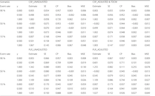
con-stant in all the models. In Table 4 and Fig. 1 we present the estimates, SEs, coverage probability, bias and MSE for the longitudinal effect on survival using the time dependent Age simulation scheme. The TDCM and the time adjusted CSP (identical results) showed lower bias and higher cover-age probability compared to the other methods. The PLR methods provided higher estimates compared to the other methods with greater bias in the unadjusted model. The es-timates for the unadjusted and the time adjusted CSP methods provide similar results in instances when the lon-gitudinal effect on survival was small. The standard errors were higher in the time adjusted models compared to the unadjusted models. The time adjusted PLR had larger standard errors and better coverage, compared to the un-adjusted PLR. When the event rate was high (90 %) and the longitudinal association with survival was high (γ= 1.000) the unadjusted PLR showed the largest bias (0.342) com-pared to other methods. The bias, though still large, was at-tenuated in the time adjusted PLR method (0.255). The unadjusted CSP showed a bias of 0.082 compared to the time adjusted CSP bias of 0.002. For lower event rates (10 %) the bias was attenuated. The unadjusted PLR showed a bias of 0.091 and the time adjusted PLR had a bias of 0.027. The unadjusted CSP also showed a bias of 0.067 compared to the time adjusted CSP bias of 0.003.
Table 3Type I error for longitudinal effect on survival
N= 1000,γ= 0a
Event rate CSP_UN CSP_AD & TDCM PLR_UN PLR_AD
90 % 0.048 0.047 0.048 0.048
50 % 0.054 0.055 0.053 0.054
10 % 0.048 0.048 0.048 0.048
a
Type I Error rate based on 10,000 simulations
Abbreviations:CSP_UNUnadjusted Cross Sectional Pooling,CSP_ADAdjusted Cross Sectional Pooling,PLR_UNUnadjusted Pooled Logistic Regression,
PLR_ADAdjusted Pooled Logistic Regression,TDCMTime Dependent Cox Regression Modeling
Table 2Summary of methods
Characteristics CSP_UN CSP_AD TDCM PLR_UN PLR_AD
Rows per subject Multiple Multiple Single Multiple Multiple
Regression model Cox Stratified Cox Cox Logistic Time adjusted logistic
Outcome Time-to-event Time-to-event Time-to-event Binary Binary
Censoring in interval permitted Yes Yes Yes No No
Time adjusted No Yes Yes No Yes
Age covariate Time varying Time varying Fixed Time varying Time varying
Sex covariate Fixed Fixed Fixed Fixed Fixed
Estimate (ratio) Hazard Hazard Hazard Odds Odds
Abbreviations:CSP_UNUnadjusted Cross Sectional Pooling,CSP_ADAdjusted Cross Sectional Pooling,PLR_UNUnadjusted Pooled Logistic Regression,PLR_AD
The PLR method also had larger standard errors compared to the Cox model in all simulation scenarios. In models with low event rates the standard errors for all methods were larger, as expected. The results suggest the time adjusted time dependent Cox regression methods performed best at estimating the association parameter compared to the unadjusted methods. The estimates were similar among the methods in instances when the longitudinal effect is weaker. In the supplement we also present the results for the comparison of the longitudinal effect on survival on sur-vival with a sample size of 100 (Additional file 1: Figure S1).
We assessed the performance of these methods in estimating the effects of Age (α1= 0.050) and Sex
(α2=−0.500). The standard errors were smaller in the
un-adjusted models compared to the time un-adjusted models. The results showed that the time adjusted PLR had a posi-tive bias in the Age effect with reduced bias when the event rate is low. The PLR methods showed a negative bias in the Sex effect compared to the other methods. The Cox models yielded reliable estimates for the Sex effect in all scenarios considered. The PLR had higher estimates for the Sex effect compared to the other methods. When the event rate was 50 %, the Age effect was similar in both the time adjusted and the unadjusted models, but with extreme event rates (10 % or 90 %) there was significant bias in the unadjusted.
These results suggest that the time adjusted Cox models provide more reliable estimates compared to the un-adjusted Cox and logistic models. In the supplement we present results for the comparison of the longitudinal effect on survival and the Age effect on survival with a sample size of 100 (Additional file 1: Table S1). We saw similar pat-terns in the results compared to a sample size of 1000 (Additional file 1: Table S2).
Application to Framingham Heart Study (FHS)
We illustrate these methods by applying them to FHS data in which lipid measurements and myocardial infarction (MI) data were collected over a period of 26 years. Since 1948 three generations of participants have been followed over the years: the Original cohort (recruited in 1948), their Offspring (recruited in 1971) and a Third Generation (recruited in 2002). Among the Offspring participants, triglycerides (TG) were measured at fairly similar time intervals of ~4 year each over a period of 26 years. The time to myocardial infarction was recorded for each participant, although some subjects were censored by the end of the study period in 2005. We log transformed the TG measures in our analysis to reduce skewness. A total of 2262 subjects with complete data were followed from 1979–2005 and data were collected at the start of each
Table 4Comparison of longitudinal effect on survival (N= 1000)
Scenarios CSP_UNADJUSTED CSP_ADJUSTED & TDCM
Event rate γ Estimate SE CP Bias MSE Estimate SE CP Bias MSE
90 % 0.000 0.003 0.054 0.957 0.003 0.006 0.003 0.055 0.954 0.003 0.006
0.500 0.498 0.055 0.954 −0.002 0.006 0.498 0.056 0.952 −0.002 0.006
1.000 1.083 0.058 0.720 0.082 0.014 1.002 0.059 0.958 0.002 0.007
50 % 0.000 −0.001 0.075 0.953 −0.001 0.011 −0.002 0.076 0.944 −0.002 0.012
0.500 0.499 0.070 0.947 −0.001 0.010 0.499 0.071 0.944 −0.001 0.010
1.000 1.001 0.073 0.946 0.001 0.011 1.002 0.074 0.948 0.002 0.011
10 % 0.000 0.007 0.168 0.944 0.007 0.058 0.007 0.171 0.938 0.007 0.060
0.500 0.501 0.158 0.947 0.001 0.051 0.501 0.161 0.946 0.001 0.053
1.000 1.067 0.145 0.906 0.067 0.048 1.003 0.147 0.937 0.003 0.045
PLR_UNADJUSTED PLR_ADJUSTED
Event rate γ Estimate SE CP Bias MSE Estimate SE CP Bias MSE
90 % 0.000 0.003 0.066 0.957 0.003 0.008 0.003 0.067 0.957 0.003 0.009
0.500 0.599 0.069 0.709 0.099 0.019 0.601 0.070 0.711 0.101 0.020
1.000 1.342 0.080 0.005 0.342 0.130 1.255 0.082 0.111 0.255 0.078
50 % 0.000 −0.001 0.080 0.950 −0.001 0.013 −0.002 0.081 0.945 −0.002 0.013
0.500 0.545 0.077 0.909 0.045 0.014 0.545 0.079 0.912 0.045 0.014
1.000 1.109 0.084 0.746 0.109 0.026 1.109 0.086 0.744 0.109 0.027
10 % 0.000 0.007 0.170 0.945 0.007 0.059 0.007 0.173 0.937 0.007 0.061
0.500 0.510 0.161 0.947 0.010 0.053 0.509 0.164 0.941 0.009 0.055
1.000 1.091 0.150 0.888 0.091 0.055 1.027 0.152 0.926 0.027 0.049
exam (Table 5). The FHS data showed a low cumulative event rate (3.71 %) for the 26-year period. In the FHS data we did see a steady increase in the TG measures from Exam 1 through Exam 6 as shown in Table 5. The mean change in TG between exams was ~ 11 mg/dL (2.40 on Natural Log Scale) with a standard deviation of ~90 mg/
dL (4.50 on Natural Log Scale). So we do not expect large fluctuations in change in the Log TG measures between the exams. A total of 177 deaths were reported (7.82 %) in FHS data. Among these deaths 35 (1.55 %) were recorded prior to cardiovascular disease. Future work considering death as competing risk or event-free composite
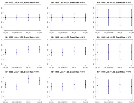
Fig. 1Estimates and Confidence Intervals for Association Parameter (N= 1000). Values are presented as estimates and 95 % confidence intervals for the link parameter. Varying link parameter (0.00, 0.50, and 1.00); varying event rates (10 %, 50 %, and 90 %). Abbreviations: CSP_UN: Unadjusted Cross Sectional Pooling; CSP_AD: Adjusted Cross Sectional Pooling; PLR_UN: Unadjusted Pooled Logistic Regression; PLR_AD: Adjusted Pooled Logistic Regression; TDCM: Time Dependent Cox Regression Modeling
Table 5Framingham heart study data (N= 2262)
Characteristics Exam 1 Exam 2 Exam 3 Exam 4 Exam 5 Exam 6
Sample size (N*) 2262 2211 2173 2118 2056 1995
Years of measurement 1979–1983 1983–1987 1987–1991 1991–1995 1995–1998 1998–2001
Age 43.32 (9.58) 47.69 (9.60) 51.15 (9.60) 54.80 (9.60) 58.87 (9.54) 61.78 (9.45)
Triglycerides 100.49 (88.77) 118.80 (123.59) 124.15 (110.18) 154.47 (133.08) 153.08 (114.92) 158.70 (112.49)
Survival time (years) 4.33 (0.60) 3.43 (0.46) 3.61 (0.46) 4.01 (0.60) 2.87 (0.86) 6.00 (1.62)
Cumulative event rate (%) 0.44 % 0.88 % 1.46 % 2.08 % 2.39 % 3.71 %
Overall event rate (%) 3.71 %
endpoints is essential in this area. In our data generation scheme and FHS data analysis we assumed missing at ran-dom (MAR) for participants who dropped out of the study with missing triglycerides at a particular exam and were censored. Additional work taking into consideration the missing data mechanism is worthy of further research.
Using the methods described in section 2 we characterize the association between the longitudinal measures and time-to-event response. We use log TG at each exam for the longitudinal part of the model assuming a linear trend over time and survival time measured from exam 1 to MI or loss to follow up. We adjust for Sex and Age in all the models. The survival distribution among subjects with the events was fairly uniform and the distribution of censored subjects was skewed with most censoring occurring at the right tail end of the distribution. In Table 6 we present the estimates for Age, Sex and the association parameters. Using a 0.05 level of significance, Age, Sex and the Log of the triglyceride measures were significantly associated with the time-to-myocardial infarction in the FHS Cohort. The association parameter describes the strength of the rela-tionship between triglycerides and MI survival;γis the log hazard ratio for a one unit increase in the longitudinal component in the survival model. The association esti-mates were similar across the different methods. The Age effect estimates and standard errors were similar among the methods. The estimates ranged from 0.048–0.056 with the unadjusted analyses yielding lower estimates compared to the time adjusted analysis. The Sex effect was also con-sistent among the different methods.
These FHS results are comparable to the simulation results with low event rate (10 %) and moderate associ-ation of the longitudinal measures to survival (γ= 0.500), as shown in Fig. 1. In this scenario, the association esti-mates were similar among the different methods.
Discussion
In this paper we explored time dependent Cox regres-sion methods that link longitudinal and survival data in order to quantify the association between a longitudinal process and a survival outcome, and have shown that statistical performance may be improved in models that explicitly include time as a covariate. We considered
models that adjust and do not adjust for time in the Pooled Logistic Regression and the Cross Sectional Pooling methods. We conducted a series of simulations to compare these methods in their ability to estimate the link param-eter. The performance was assessed through bias, coverage probabilities and Type I error rates. We analyzed data from FHS in which triglyceride measurements and Myocardial Infarction (MI) data were collected over a period of 26 years (1979–2005). To our knowledge this is the first paper that compares time adjusted and unadjusted models for modeling time dependent covariate data.
From the simulations we see that time adjusted, time dependent Cox regression methods performed best at estimating the association parameter compared to the unadjusted Cox and logistic models. Our results indicate that in some instances the PLR provides higher biased estimates and standard errors compared to the Cox models. The PLR and the time dependent Cox regres-sion methods provide similar results when the event is rare, consistent with the results presented by Green and Symons [10]. In the unadjusted models the Age effect was attenuated depending on the association of the lon-gitudinal measures on survival. D’Agostino et al. [6] indi-cated that the analyst must consider the nature of variables such as Age, which may be highly correlated with the follow-up time. There are a number of recent epidemiologic studies that implement the PLR model. Some recent work include Miguel-Yanes et al. [19]; Meigs et al. [20]; Fox et al. [21]; Ficociello et al. [22]., Marshall et al. [23]., Solomon et al. [24]. Recent studies that have also implemented the CSP approach include Schnabel et al. [25]., Magnani et al. [26]., Rienstra et al. [27]., D'Agostino [28]. The TDCM and stratified Cox model are more routine in statistical analysis. The imple-mentation of time adjustment in PLR models is essential to obtain reliable estimates.
The FHS sample provided results that were consistent with the simulation results for a low event rate and moderate association. Thus, we did not find large differ-ences in the estimates from the different approaches. Had the event rates been high and there were a strong association between the longitudinal measures and the survival time, we would have expected to see greater
Table 6Modeling longitudinal and survival data (framingham heart study)
AGE (α1) SEX (α2) LogTG (γ)
Methods Estimate SE P Estimate SE P Estimate SE P
CSP Unadjusted 0.0528 0.0103 <.0001 −1.0305 0.2434 <.0001 0.6068 0.1732 0.0005
CSP Adjusted & TDCM 0.0561 0.0119 <.0001 −1.0254 0.2435 <.0001 0.6182 0.1741 0.0004
PLR Unadjusted 0.0480 0.0101 <.0001 −1.0179 0.2444 <.0001 0.6023 0.1754 0.0006
PLR Adjusted 0.0520 0.0119 <.0001 −1.0154 0.2444 <.0001 0.6107 0.1755 0.0005
Abbreviations:CSP_UNUnadjusted Cross Sectional Pooling,CSP_ADAdjusted Cross Sectional Pooling,PLR_UNUnadjusted Pooled Logistic Regression,PLR_AD
differences in the estimates from the unadjusted models, with the time-unadjusted PLR and CSP approaches hav-ing higher estimates.
There is extensive literature on comparison of the lo-gistic regression model and the proportional hazard model. Efron [15] discusses the use of the logistic model for survival data and shows that the odds ratio estimates are approximately the same as hazard ratios. Green and Sy-mons [10] conducted research on the conditions under which results from the Logistic regression and proportional hazards model in prospective epidemiologic studies ap-proximate one another. They concluded that in instances where the follow-up period is short and the disease is gen-erally rare, the regression coefficients of the logistic model approximate those of the proportional hazards model with a constant underlying hazard rate. They also stated that under the same conditions the regression coefficients have similar estimated standard errors. They provided a math-ematical relationship between the Cox and the logistic models. D‘Agostino et al. [6] showed that the pooled logistic regression (PLR) is close to the time dependent covariate model. They also provided numerical examples showing the closeness of this relationship using the Framingham Heart Study. The goal of our paper was to compare these methods using simulation studies considering models that adjust and do not adjust for time in PLR and CSP and also illustrate instances where these methods differ.
In time dependent covariate models attention has to be placed on the type of covariates (internal vs. external) ing considered. Kalbfleisch & Prentice [12] distinguish be-tween external and internal covariates, where an external covariate does not require direct observation of the indi-vidual. Examples are the age of an individual and level of air pollution as a risk factor for asthma attacks. Internal covariates are generated within the individuals under study and are known only when the individual remains in the study as event-free and is uncensored. As noted by Kalbfleisch and Prentice, internal covariate processes can be affected by treatment assignment in clinical trials, or by baseline factors in observational studies such as the Fra-mingham Heart Study. In such instances care must be exercised in the interpretation, as treatment or baseline covariate effects may be reflected predominantly in the time-varying covariate process [12]. We acknowledge the potential limitations of predicting survival with internal time-varying covariates given the conceptualization of the conditional survival function; however, we used internal time-dependent covariates in our Framingham Heart Study example given the clinical interest in the relation-ship between TG values and risk of myocardial infarction. Thus care needs to be taken in the interpretation of the results given the use of an internal time-varying factor that may also be an intermediate variable between the baseline factors and the outcome.
One limitation to our study is that we did not consider measurement errors or missing data issues that may arise from longitudinal covariate data that are potentially missing at failure times. In many longitudinal studies participants may drop out early from the study which may lead to missing data in both the failure times as well as the time dependent covariates. Such issues can be addressed in a mixed effects model in which a random effect can be used to capture the individual specific lon-gitudinal trajectories with missing data. Complete-case methods, which discard incomplete observations in sur-vival regression models, may potentially lead to ineffi-cient or biased estimates. In the presence of missing data, there are a number of likelihood and imputation methods for addressing missing data given the observed data. In our study we did not address these issues as our simulations and examples are based on no missing data at each time point. Models that consider measurement error may be more representative of the underlying process. In our study, using Framingham Heart Data, individuals were censored at time of death. A drawback to this approach is that death without prior myocardial infarction may be considered a competing event to our outcome. The main objective of our study was to present an overview of these methods for modeling time dependent covariates in the context of longitudinal and survival data. Exploring methods that consider death as competing risk or event-free composite endpoints are worthy of further research. A limitation to every simulation study is that the results are dependent on the scenarios examined. In this paper, we evaluated a range of models to provide broader insight, but our conclusions must be limited to the scenarios that we examined. In the simulation models the assumption of proportional hazards was considered in all scenarios. Fur-ther work is needed to better understand the circum-stances when the PLR may differ from Cox models in non-proportional hazard models.
Conclusions
of the available data compared to the PLR by including time. Thus, when time is available, we recommend using the TDCM or equivalently the stratified CSP approaches with time intervals. Survival analyses that explicitly ac-count for the times at which time dependent covariates are measured appear to provide more reliable estimates compared to unadjusted analyses.
Additional file
Additional file 1: Figure S1.Estimates and Confidence Intervals for Association Parameter (N= 100). Values are presented as estimates and 95 % confidence intervals for the link parameter. Varying link parameter (0.00, 0.50, and 1.00); varying event rates (10 %, 50 %, and 90 %). Abbreviations: CSP_UN: Unadjusted Cross Sectional Pooling; CSP_AD: Adjusted Cross Sectional Pooling; PLR_UN: Unadjusted Pooled Logistic Regression; PLR_AD: Adjusted Pooled Logistic Regression; TDCM: Time Dependent Cox Regression Modeling. (DOCX 84 kb)
Abbreviations
CSP:Cross sectional pooling; CSP_AD: Adjusted Cross-sectional pooling; CSP_UN: Unadjusted Cross-sectional pooling; FHS: Framingham Heart Study; MI: Myocardial Infarction; MSE: Mean square error; PLR: Pooled Logistic Regression; PLR_AD: Adjusted Pooled logistic regression;
PLR_UN: Unadjusted Pooled logistic regression; TDCM: Time dependent covariate modeling; TG: Triglycerides
Acknowledgements
We thank Dr. Timothy Heeren for his input in the simulation analysis.
Funding
This work was supported by the National Heart, Lung and Blood Institute's Framingham Heart Study (Contracts N01-HC-25195 and HHSN268201500001I) of the National Institutes of Health and Boston University School of Medicine. A portion of this research was conducted using Boston University Linux Cluster for Genetic Analysis (LinGA) funded by the National Center for Research Resources (NIH NCRR).
Availability of data and materials
The data used in this study are available at NIH BioLINCC (https:// biolincc.nhlbi.nih.gov/home/). They can also be provided to interested researchers on written request to FHS. Request for FHS data may be done by submitting a proposal through the FHS web-based research application. A catalogue of the FHS data repository may be accessed through the FHS website: www.framinghamheartstudy.org/researchers/description-data/.
Authors’contributions
JSN, MJP and LAC conceived the study. The data were cleaned by JSN and LAC. All authors contributed towards the design of the simulation scenarios implemented in the study. The analysis was carried out by JSN. The manuscript was written by JSN. All authors contributed toward reviewing and revising the final manuscript. All authors read and approved the final manuscript.
Competing interests
The authors declare that they have no competing interests.
Consent for publication
Manuscript does not contain any individual person’s data.
Ethics approval and consent to participate
The research protocols of the FHS are reviewed annually by the Institutional Review Board of the Boston University Medical Center and by the Observational Studies Monitoring Board of the National Heart, Lung and Blood Institute. Since 1971, written consent has been obtained from participants before each examination. Information about the content of the Framingham Heart Study research examinations is presented to the participants at each examination cycle in the text of the corresponding consent form and in a discussion with a
trained admitting coordinator at the beginning of the scheduled appointment. Information from every completed consent form is coded and recorded in a database. Questions regarding the ethical conduct of research are presented by FHS investigators to the FHS Ethics Advisory Board. The Advisory Board reviews, discusses, and make recommendations regarding these questions.
Author details
1
Department of Biostatistics, Boston University, School of Public Health, 801 Massachusetts Ave, CT 3rd Floor, Boston, MA 02118, USA.2Department of Biostatistics, Johns Hopkins Bloomberg School of Public Health, 615 North Wolfe St, Baltimore, MD 21205, USA.3Department of Biostatistics and Bioinformatics, Duke University, School of Medicine, 2400 Pratt St, 7021 North Pavilion, Durham, NC 27705, USA.4National Heart, Lung, and Blood Institute’s Framingham Heart Study, Framingham, MA 01702, USA.
Received: 14 March 2016 Accepted: 17 October 2016
References
1. Fisher LD, Lin DY. Time dependent covariates in the Cox proportional-hazards regression model. Annu Rev Public Health. 1999;20(1):145–57. 2. Cox DR, & Oakes D. Analysis of survival data (Vol. 21). London: CRC Press;
1984.
3. Therneau TM, Grambsch PM. Modeling survival data: extending the Cox model. Berlin: Springer Science & Business Media; 2000.
4. Cox DR. Regression models and life-tables. J R Stat Soc Ser B (Methodological). 1972;187–220.
5. Cupples LA, D'Agostino RB, Anderson K, Kannel WB. Comparison of baseline and repeated measure covariate techniques in the Framingham Heart Study. Stat Med. 1988;7(1–2):205–18.
6. D'Agostino RB, Lee ML, Belanger AJ, Cupples LA, Anderson K, Kannel WB. Relation of pooled logistic regression to time dependent Cox regression analysis: The Framingham Heart Study. Stat Med. 1990;9(12):1501–15. 7. Pepe MS, Cai J. Some graphical displays and marginal regression analyses
for recurrent failure times and time dependent covariates. J Am Stat Assoc. 1993;88(423):811–20.
8. Prentice RL, Gloeckler LA. Regression analysis of grouped survival data with application to breast cancer data. Biometrics. 1978;34:57–67.
9. Abbott RD. Logistic regression in survival analysis. Am J Epidemiol. 1985; 121(3):465–71.
10. Green MS, Symons MJ. A comparison of the logistic risk function and the proportional hazards model in prospective epidemiologic studies. J Chron Dis. 1983;36(10):715–23.
11. Ingram DD, Kleinman JC. Empirical comparisons of proportional hazards and logistic regression models. Stat Med. 1989;8(5):525–38.
12. Kalbfleisch JD, Prentice RL. The statistical analysis of failure time data (Vol. 360). New York: John Wiley & Sons; 2011.
13. Wu M, Ware JH. On the use of repeated measurements in regression analysis with dichotomous responses. Biometrics. 1979;35:513–21. 14. Wu L. Mixed effects models for complex data. London: CRC Press; 2010. 15. Efron B. Logistic regression, survival analysis, and the Kaplan-Meier curve.
J Am Stat Assoc. 1988;83(402):414–25.
16. Allison PD. Survival analysis using SAS: a practical guide. Cary NC: Sas Institute; 2010.
17. Singer JD, Willett JB. Applied longitudinal data analysis: Modeling change and event occurrence. Oxford: Oxford university press; 2003.
18. Burton A, Altman DG, Royston P, Holder RL. The design of simulation studies in medical statistics. Stat Med. 2006;25(24):4279–92.
19. De Miguel-Yanes JM, Shrader P, Pencina MJ, Fox CS, Manning AK, Grant RW, Meigs JB. Genetic risk reclassification for type 2 diabetes by age below or above 50 years using 40 type 2 diabetes risk single nucleotide polymorphisms. Diabetes Care. 2011;34(1):121–5.
20. Meigs JB, Shrader P, Sullivan LM, McAteer JB, Fox CS, Dupuis J, Cupples LA. Genotype score in addition to common risk factors for prediction of type 2 diabetes. N Engl J Med. 2008;359(21):2208–19.
21. Fox CS, Pencina MJ, Meigs JB, Vasan RS, Levitzky YS, D’Agostino RB. Trends in the Incidence of Type 2 diabetes mellitus from the 1970s to the 1990s The Framingham Heart Study. Circulation. 2006;113(25):2914–8. 22. Ficociello LH, Perkins BA, Silva KH, Finkelstein DM, Ignatowska-Switalska H,
patients who have type 1 diabetes and are treated with angiotensin-converting enzyme inhibitors. Clin J Am Soc Nephrol. 2007;2(3):461–9. 23. Marshall LM, Spiegelman D, Barbieri RL, Goldman MB, Manson JE, Colditz GA,
Hunter DJ. Variation in the incidence of uterine leiomyoma among premenopausal women by age and race. Obstet Gynecol. 1997;90(6):967–73. 24. Solomon DH, Karlson EW, Rimm EB, Cannuscio CC, Mandl LA, Manson JE,
Curhan GC. Cardiovascular morbidity and mortality in women diagnosed with rheumatoid arthritis. Circulation. 2003;107(9):1303–13.
25. Schnabel RB, Sullivan LM, Levy D, Pencina MJ, Massaro JM, D'Agostino RB, Kannel WB. Development of a risk score for atrial fibrillation (Framingham Heart Study): a community-based cohort study. Lancet. 2009;373(9665):739–45. 26. Magnani JW, Moser CB, Murabito JM, Nelson KP, Fontes JD, Lubitz SA,
Benjamin EJ. Age of natural menopause and atrial fibrillation: The Framingham Heart Study. Am Heart J. 2012;163(4):729–34.
27. Rienstra M, Lyass A, Murabito JM, Magnani JW, Lubitz SA, Massaro JM, Benjamin EJ. Reciprocal relations between physical disability, subjective health, and atrial fibrillation: The Framingham Heart Study. Am Heart J. 2013;166(1):171–8. 28. D'Agostino RB. Beyond baseline data: the use of time-varying covariates.
J Hypertens. 2008;26(4):639–40.
• We accept pre-submission inquiries
• Our selector tool helps you to find the most relevant journal
• We provide round the clock customer support
• Convenient online submission
• Thorough peer review
• Inclusion in PubMed and all major indexing services
• Maximum visibility for your research
Submit your manuscript at www.biomedcentral.com/submit