Hierarchical level features based trainable segmentation for electron microscopy images

(1)

R E S E A R C H

Open Access

Hierarchical level features based trainable

segmentation for electron microscopy images

Shuangling Wang

1

, Guibao Cao

1

, Benzheng Wei

2

, Yilong Yin

1*

, Gongping Yang

1

and Chunming Li

3

* Correspondence:[email protected] 1

School of Computer Science and Technology, Shandong University, Jinan 250101, China

Full list of author information is available at the end of the article

Abstract

Background:The neuronal electron microscopy images segmentation is the basic and key step to efficiently build the 3D brain structure and connectivity for a better understanding of central neural system. However, due to the visual complex appearance of neuronal structures, it is challenging to automatically segment membranes from the EM images.

Methods:In this paper, we present a fast, efficient segmentation method for neuronal EM images that utilizes hierarchical level features based on supervised learning. Hierarchical level features are designed by combining pixel and superpixel information to describe the EM image. For pixels in a superpixel have similar characteristics, only part of them is automatically selected and used to reduce information redundancy. To each selected pixel, 34 dimensional features are extracted by traditional way. Each superpixel itself is viewed as a unit to extract 35 dimensional features with statistical method. Also, 3 dimensional context level features among multi superpixels are extracted. Above three kinds of features are combined as a feature vector, namely, hierarchical level features to use for

segmentation. Random forest is used as classifier and is trained with hierarchical level features to perform segmentation.

Results:In small sample condition and with low-dimensional features, the

effectiveness of our method is verified on the data set of ISBI2012 EM Segmentation Challenge, and its rand error, warping error and pixel error attain to 0.106308715, 0.001200104 and 0.079132453, respectively.

Conclusions:Comparing to pixel level or superpixel level features, hierarchical level features have better discrimination ability and the proposed method is promising for membrane segmentation.

Keywords:Machine learning, Biomedical image processing, Hierarchical level features, Random Forest, Membrane segmentation

Introduction

In order to get new insights into the functional structure of the brain, neuroanatomists need to reconstruct and mapping neural connections in 3D, which the key approach is 2D neuron image segmentation. Currently, electron microscopy (EM) is the main im-aging tool which can provide sufficient resolution for studying connections at the neuron level. EM enables acquisition of huge datasets, which make tedious and time-consuming manual analysis simply infeasible. Therefore, accurately automatic neuronal segmentation is naturally proposed to resolve this problem. However, the intricate cell

© 2013 Wang et al.; licensee BioMed Central Ltd. This is an Open Access article distributed under the terms of the Creative Commons Attribution License (http://creativecommons.org/licenses/by/2.0), which permits unrestricted use, distribution, and reproduction in any medium, provided the original work is properly cited.

(2)

textures and structures with largely varying shapes and topologies, etc. [1] make the automatic segmentation of neuronal EM images very challenging. Figure 1 shows two slices of EM images.

In previous works of membrane segmentation in EM images, two trends deserve pay-ing much more attention. One is that more and more supervised machine learnpay-ing methods are used. The other is to find more discriminative feature for segmentation. As to feature extraction for membrane segmentation in EM images, related works can be divided into two categories, namely implicit methods and explicit ones.

Implicit methods usually deployed deep learning paradigm, in which raw pixel inten-sities are often directly used as the input to train artificial neural network (ANN) or its variants. This paradigm can learn features automatically and effectively. Authors in [2] sampled raw pixel intensities from fixed size rectangular window to train a multilayer Convolutional Neural Network (CNN) [3] to segment membranes. Neuron membranes were detected in [4] by using a serial ANN architecture combined with a feature vector composed of image intensities sampled from a special stencil neighborhood. In this frame-work, classifiers are trained in sequential order and each ANN is allowed to use the classi-fication result of the prior one as a part of the input. In [5] multi-scale stencil windows and radon-like features are used to learn a series of discriminative models to detect neuron membranes in EM Images. A special deep ANN is adopted by authors [6] as a pixel classifier and the label of each pixel is predicted from raw pixel values in a square window centered on it. In this method, each window pixel is mapped to a neuron in the input layer, followed by a succession of convolutional and max-polling layers.

As to explicit methods, image features are predefined before classifier is learned. In [7] the importance of context information for membrane segmentation is highlighted by using local context features computed from the hessian matrix to train a boosted classifier. The neighborhood is defined by a star shaped stencil with 8 arms (see Figure 2). By finding global dense correspondence between two sections, authors [8] exploited context information from the neighboring sections to reduce the ambiguities in neuronal segmentation of a section and extracted pixel level features to train a ran-dom forest classifier.

(3)

Although existed works achieve a reasonable segmentation result, they still have some challenges as following:

(1.) They tend to obtain context information sampled on rectangular (see Figure3) or predefined stencil window (see Figure2). Obviously such windows of fixed size or shape are inconsistent with the natural boundaries of images and one window may cover several distinct image regions. It will degrade the

segmentation accuracy [9].

Figure 2Stencil neighborhood.The stencil neighborhood is defined by a star shaped template with its 8 arms forking out every 45 degree.

Figure 3Rectangular window-based neighborhood vs superpixel-based neighborhood.Rectangular windows fail to correctly identify the boundaries of original images while superpixels preserve original image boundaries and enforce local consistency.

Wanget al. BioMedical Engineering OnLine2013,12:59 Page 3 of 14

(4)

(2.) In order to get more discriminative context information, deep learning methods often adopt a large window, so that classifier training is computational intensive.

(3.) It is sensitive to noise and time consuming to implement segmentation only with pixel level features. Also, pixel level features could not describe local consistency characteristic of EM images.

Obtained by grouping nearby pixels, superpixel is a natural form of enforcing local consistency while respecting original image boundaries. Recent studies on superpixels showed that superpixels had superior performance to using rectangular image win-dows for localized image processing [9-11]. Moreover, superpixel, as a visual primi-tive, performs high efficiency for classification. For example, [11] gave a fully automated approach to segment mitochondria by using superpixel-based shape and local features. [10] performed automated nuclear segmentation by coupling superpixel context information with artificial neural networks. Although superpixel classifier is efficient, superpixel label is sensitive to the granularity of grouping. So superpixel classifier for EM images might be suitable for shaped and unconnected organelles segmentation.

Comparing to pixel, superpixel is a bigger granularity representation of the image. Pixels inside a superpixel have similar attributes, which is in reasonable agreement with the characteristic of local clustering of neuronal EM images. Superpixel-based features can be regarded as a kind of mid-level features, and pixel-based features as a kind of low level features. A natural idea is that superpixel level features may have different discriminative information from pixel level features for segmentation and the two kinds of features should be complementary at some degree. Superpixels nat-urally with the local information can be as a new formulation of adaptive windows neighborhood.

In the view of the above consideration, we define hierarchical level features which consist of pixel level features, superpixel level features and context level features among multi superpixels and random forest is used as classifier and is trained with hierarchical level features to perform segmentation. The effectiveness of our method is verified on the data set of ISBI2012 EM Segmentation Challenge.

Methods

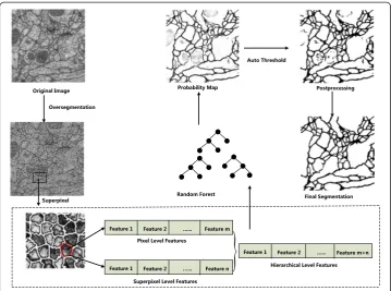
Framework based upon the proposed hierarchical level features and random forest for membrane segmentation is provided in the beginning of this section. Later, three import-ant steps in this work, namely, preprocessing, trainable segmentation and postprocessing are presented. In the step of preprocessing, one newly proposed but widely used superpixel oversegmentation algorithm is introduced. In the stage of trainable segmenta-tion, hierarchical level feature definition and extraction are given and Random Forest is used to implement segmentation.

Figure 4 provides an overview of our method, and our method consists of the following three steps:

I. Preprocessing: image enhancement, superpixel oversegmentation

(5)

Preprocessing

Before oversegmentation and feature extraction, images were preprocessed with histo-gram equalization and Gaussian filter to reduce noise, make the intensity more uniform and improve the contrast of the membranes.

Superpixel oversegmentation

Image oversegmentation is a usual way to obtain superpixels, and superpixels demon-strate local clustering of images. Obtained by the nearby pixel grouping, superpixels might be a more natural and perceptually meaningful representation of reality [12]. It has been shown that using superpixels are advantageous because they can preserve natural image boundaries and reduce redundant information of the image data as well as enforce local consistency [11].

In this work, we apply Simple Linear Iterative Clustering (SLIC) [13] to generate superpixels, which is a variant of k-means algorithm. By integrating the local intensity and position information, SLIC divides an image into small patches. Superpixels obtained by SLIC are nearly uniform size and their boundaries are closely match true image boundaries. In addition, SLIC only need specify one parameter of the desired number of superpixels and has low computation complexity.

SLIC has with two important distinctions:

1. SLIC searches a limited region proportion to the superpixel size. S¼pffiffiffiffiffiffiffiffiffiN=k, where

sis the grid interval, N is the number of pixels, andkis the desired number of superpixels. A superpixel is a region of approximate sizes×s,the search for similar pixels is done in a region 2s× 2saround the superpixel center.

2. SLIC adopts a weighted distance measureD,as shown in Equations (1)-(3). Figure 4Overview of our method.

(6)

a. SLIC clusters pixels in the combined five dimensional color and image plane space to efficiently generate compact, nearly uniform superpixels.

ds¼

ffiffiffiffiffiffiffiffiffiffiffiffiffiffiffiffiffiffiffiffiffiffiffiffiffiffiffiffiffiffiffiffiffiffiffiffiffiffiffi

xj−xi

2

þ yj−yi

2

r

ð1Þ

dc¼

ffiffiffiffiffiffiffiffiffiffiffiffiffiffiffiffiffiffiffiffiffiffiffiffiffiffiffiffiffiffiffiffiffiffiffiffiffiffiffiffiffiffiffiffiffiffiffiffiffiffiffiffiffiffiffiffiffiffiffi

lj−li

2

þ aj−ai

2

þ bj−bi

2

q

ð2Þ

D¼

ffiffiffiffiffiffiffiffiffiffiffiffiffiffiffiffiffiffiffiffiffiffiffiffiffiffiffiffiffiffiffiffiffi

dc Nc

2

þ ds Ns

s

ð3Þ

where [l a b]Tdenotes color space, [x y]Tdenotes the pixel’s position, [lk,ak,bk,xk,yk]T

de-notes cluster center,dsis space proximity,dcis color proximity, andNc, Nsare the

nor-malized factors.

Trainable segmentation

Superpixel based automatic representative sample selection

For large volumes of EM data set, training pure pixel classifier is large time consuming and big storage space demanding. Pixels inside the same superpixel can be seen as homogenous, thus there are similarity and redundancy between pixels. So we apply superpixel based automated representative sample selection. Specifically, in each superpixel, we apply certain criterions (for example choosing points randomly) to select pixel samples to represent all the pixels inside this superpixel (see Figure 5). For simpli-city, we just randomly select one point corresponding to one single superpixel in our work. Besides, this automated sample selection is robust to noise.

Hierarchical level features (HLFs)

Low level features extraction (pixel-based features extraction) Most of pixel

fea-tures are provided by Fiji with default parameters (http://fiji.sc/wiki/index.php/About). Fiji is a public software package for feature extraction. Our set of 34-dimensional pixel features is as following: (1) 6-dimensional filter values with 3*3 neighborhood: Mean, Median, Maximum, Minimum, Variance, Gaussian blur. (2) Gaussian filter values with Sigma 1.5, 2.0, 3.5, 4.0, 5.0, and 6.0, respectively. Sobel filter with 3*3 kernel size, Lar-gest Hessian and Smallest Hessian, Difference of Gaussian, Linear Kuwahara, Laplacian, Largest Structure and Smallest Structure, Derivative. In addition, we incorporate 12-dimensional ray features [14] and 1-12-dimensional Radon-like feature [15], which are newly developed and proved to be informative for neuronal reconstruction. Selected features are depicted in Figure 6.

Mid-level features extraction (superpixel-based features extraction) From the

(7)

Figure 5Automatic training point selection.Red points denotes selected points, and for illustration, one point corresponding to one superpixel.

Original Image Enhanced Image Maximum Filter Derivative

Edge Largest structure Laplacian Largest hessian

Figure 6Selected examples of extracted features.

(8)

the superpixel features with statistical methods are twofold: First, there are rich pixel level features, thereby using statistical methods for superpixel feature extraction greatly enriches the representations of superpixel. Second, many statistical methods such as mean, variance are simple and efficient. In this paper, we represent a superpixel by sim-ply averaging various pixel level features, thus we can get 34-dimensional superpixel features. And superpixel entropy derived from superpixel intensity histogram is utilized as one dimension of superpixel features. In addition, we also use 3-dimensional context level features among multi superpixels, such as mean intensity, mean gradient, intensity variance of neighboring superpixels.

In total, we use 35-dimensional superpixel features and 3-dimensional superpixel context information. In fact, context level features among multi superpixels belong to superpixel level features.

Integrate low level features with mid-level features as the HLFs To each pixel, we

get its superpixel-based neighborhood, which is different from conventional rectangular window-based neighborhood. And the new method is not only naturally adaptive but also has more perceptual meaningful. In total, we utilize 72-dimensional features, in which there are 34-dimensional pixel features, 35-dimensional superpixel features and 3-dimensional superpixel context information.

Classification

After selecting a set of features, another important step is to select a good classifier. Random forest is a widely employed “ensemble learning” method for classification and regression proposed by Breiman. This method is robust and user-friendly as it has only two parameters and it can work efficiently on large data sets. Even in presence of many noisy features, Random Forest works well, so it is unnecessary to perform feature selec-tion procedure. Considering all of the above, we adopt Random Forest to train the pro-posed HLFs.

Random forest is ensemble learning consists of tree predictors such that each tree depends on the values of a random vector sampled independently and with the same distribution for all trees in the forest [16]. Each tree is grown as follows: First, the best split at each node is selected from among a random subset of the predictor vari-ables. Different variables are used at each split in different trees. Second, the training set used to grow each tree is a bootstrap sample of the observations, i.e., a sample of sizeNdrawn with replacement from the original sample ofNobservations. Some servations are represented multiple times, while others are left out. The left-out ob-servations are called “out-of-bag” and are used to estimate prediction error, eliminating the need for a test set or cross-validation. Third, each tree is grown to its large extent possible, and there is no pruning. The random forests final prediction is the mean prediction (regression) or class with maximum votes (classification). Breiman [16] showed that the prediction error converges to a limiting value as the number of trees tends to infinity.

Postprocessing

(9)

removing, performed by a series of thresholding operations based on region properties such as Area, Euler Number, Solidity and Eccentricity.

Experiments and results Description of the data set

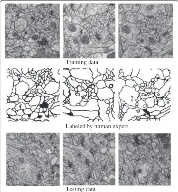
The data we used in this paper provided by the organizers of the ISBI 2012 EM Seg-mentation Challenge (http://www.biomedicalimaging.org/2012/index.php). The data set consists of training data and testing data of the Drosophila first instar larva ventral nerve cord, which is provided in the form of EM stack.

The training data labeled by an expert human neuroanatomist is a set of 30 sections from a serial section Transmission Electron Microscopy (ssTEM) data set. The test data (ground truth unknown to the authors) consisting of 30 sections is another volume from the same Drosophila first instar larva ventral nerve cord. Some typical slices and their corresponding labels are depicted in Figure 7.

Training data

Labeled by human expert

Testing data

Figure 7Selected slices of training data, corresponding label and test data.

(10)

Evaluation metrics

Segmentation result for challenge is evaluated through an automated online system; the system computes three error metrics in relation to the hidden ground truth: pixel error, warping error and the Rand error.

Pixel error

It is defined as 1 - the maximal F-score of pixel similarity or squared Euclidean distance between the original and the result labels [17].

Warping error

The warping error is segmentation metric that tolerates disagreements over boundary location, penalizes topological disagreements, and can be used directly as a cost func-tion for learning boundary detecfunc-tion [17].

Rand error

The Rand error metric is based on the Rand index, defined as 1 - the maximal F-score of Rand index [18], a measure of similarity between two clusters or segmentations. It has a more intuitive interpretation, but completely disregards non-topological errors [6].

Comparison experiments on different level features

We do experiment to compare the segmentation performance of pure pixel, pure superpixel and HLFs on the three metrics.

Experimental setting

We divide the public training data set into two parts: previous 15 sections as our training set, remaining 15 sections as our test set. In order to test the effect of superpixel size on classification accuracy, we set the parameter of superpixel number for each section of EM image ranging from 7500 to 11500. For simplicity, just one single pixel point is randomly selected corresponding to one superpixel.

Classification results

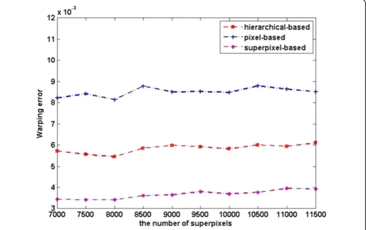
The quantitative segmentation results of the three kinds of level features are shown in Figures 8, 9, and 10.

(11)

The plots in Figure 8 show the pixel error on the dataset. We can see from the plots that pixel level features perform better than superpixel level ones. This can be explained as pixel level features have richer information than superpixel level ones, as a result the image can be represented better by pixel level features. Pixel error plot of superpixel level features shows an upward trend with the increasing of number of superpixels, this is because classification at superpixel level is sensitive to granu-larity of oversegmentation. However, superpixel based segmentation performs bet-ter in warping error, see Figure 10, this is due to superpixel inherently adheres

Figure 9Rand error of different level features.

Figure 10Warping error of different level features.

(12)

well to the original image boundaries. Rand error plots in Figure 9 clearly demon-strate the substantial improvement in the segmentation by our method. We can draw a conclusion from Figures 9 and 10 that our method integrates the advan-tages of pixel level feature and superpixel level features.

HLFs feed into different learning algorithms

Aim to validate the recognition performance of HLFs as well as to find the best suit-able classifier, we conduct experiments for different learning algorithms supplied with HLFs. We choose several currently popular classifiers: Random Forest (RF), Support Vector Machine (SVM) [19], AdaBoost [20] as well as Linear classifier. All the classifiers are trained with default parameters. In this experiment, training set and testing set are similar to the previous experiment, and number of superpixel is 8000 for each image. Experiment results are showed in Table 1.

From Table 1 we can see that HLFs-RF achieves the best segmentation performance in general. Due to all results are directly returned by classifier without any postprocessing and rand error is very sensitive to topological errors, rand error for all the four methods is not good enough. Training set is not sufficient, which is maybe another reason for the lower rand error. SVM performs well for segmentation in pixel error, while rand error is quite poor. We explain this as SVM works well for problem in small sample condition and balanced data. It can be stated that RF is the better clas-sifier suitable for the membrane segmentation.

Computational time

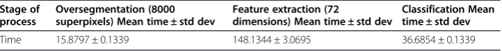
All the experiments are performed on a computer with a Core i7 950 3.06GHz pro-cessor, 24GB of RAM, and four GTX 580 graphics cards and implemented in MATLAB. For the HLFs-RF method, we computed the average computational time (in seconds) of one image with standard deviation in different stage of the proposed method. The statistical result is shown in Table 2.

From Table 2 we can see that the average computational time of one image with our method is about 201 seconds and it can basically satisfy actual application. Table 1 Different learning algorithms supplied with HLFs

Method Rand error Warping error Pixel error

HLFs-SVM 0.81862738 0.00482126 0.06570173

HLFs-AdaBoost 0.71340669 0.00370051 0.07302954

HLFs-Linear 0.41051885 0.00756352 0.13368690

HLFs-RF 0.29548843 0.00282007 0.09258893

Table 2 Average computational time for one image (in seconds) in different stage of HLFs-RF

Stage of process

Oversegmentation (8000 superpixels) Mean time ± std dev

Feature extraction (72

dimensions) Mean time ± std dev

Classification Mean time ± std dev

(13)

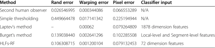
The comparison experiment on the data set of ISBI2012

In this section, we compare our method with the two benchmark methods of ISBI2012 competition, namely Second Human Observer and Simple Thresholding, as well as two newly published methods of [8] and [21]. 1878 dimension features are used in Laptev’s method, while only 72 dimension features are used in our method. In addition, only part of pixels in each superpixel is used in our method, which means small sample condition.

Experimental results are shown in Table 3. Even with quite low dimensional fea-tures and in small sample condition, our method still shows better performance comparing to other four existed ones on the whole. It indicates that HLFs have more discriminative ability than pixel level features.

Conclusions and future work

This paper deals with the segmentation of neuronal structures in EM stacks based on supervised learning method. Considering the local clustering of neuronal EM images, we define and extract HLFs, which can be regarded as kind of more reason-able and natural feature representation, and use Random Forest as a classifier to im-plement segment of membranes with HLFs. Experimental validation demonstrates a promising performance of our method.

Future works will focus on two directions. One is to find more discriminative fea-ture representation for superpixel. The other is to develop new classification tech-niques so that HLFs can be more fully utilized.

Abbreviations

HLFs:Hierarchical Level Features; ISBI: IEEE International Symposium on Biomedical Imaging; EM: Electron Microscopy; ANN: Artificial Neural Network; CNN: Convolutional Neural Network; SLIC: Simple Linear Iterative Clustering; ssTEM: Serial section Transmission Electron Microscopy; RF: Random Forest; SVM: Support Vector Machine.

Competing interests

The authors declare that they have no competing interests.

Authors_’contributions

SW designed the proposed method and drafted the manuscript. Implementation and experiment results analysis were done by GC. BW helped in drafting the manuscript. YY supervised the project, contributed to discussion and analysis and participated in manuscript revisions. GY and CL participated in manuscript revisions and provided critical review that helped in improving the manuscript. All authors read and approved the final manuscript.

Acknowledgements

The work is supported by NSFC Joint Fund with Guangdong under Key Project U1201258, Program for New Century Excellent Talents in University of Ministry of Education of China (NCET-11-0315), and the Natural Science Foundation of Shandong Province (NO.ZR2011FQ033).

Table 3 Experimental results of several methods on the ISBI2012’s data set

Method Rand error Warping error Pixel error Classifier input

Second human observer 0.026546995 0.000344086 0.066553289 N/A Simple thresholding 0.449664478 0.017141342 0.225194944 N/A

Laptev’s method – 0.00062 0.079264809 1878 dimension features

Burget’s method 0.139038440 0.002641296 0.102285508 Local-level and Segment-level features HLFs-RF 0.106308715 0.001200104 0.079132453 72 dimension features

“–”means unknown, [Laptev et al., MICCAI’2012] do not indicate the Rand error. N/A means not available.

(14)

Author details 1

School of Computer Science and Technology, Shandong University, Jinan 250101, China.2College of Science and Technology, Shandong University of Traditional Chinese Medicine, Jinan 250355, China.3_{Department of Radiology,}

University of Pennsylvania, Philadelphia, PA 19104, USA.

Received: 14 May 2013 Accepted: 19 June 2013 Published: 28 June 2013

References

1. Liu T, Jurrus E, Seyedhosseini M, Ellisman M, Tasdizen T:Watershed merge tree classification for electron microscopy image segmentation.Pattern Recognition (ICPR)2012:133–137. 21st Internarional Conference on, Tsukuba, Japan.

2. Jain V, Murray JF, Roth F, Turaga S, Zhigulin V, Briggman KL, Helmstaedter MN, Denk W, Seung HS:Supervised learning of image restoration with convolutional networks.InComputer vision, 2007 ICCV 2007 IEEE 11th international conference on Rio de Janeiro.Brazil: IEEE; 2007:1–8.

3. LeCun Y, Bengio Y:Convolutional networks for images, speech, and time series.InThe handbook of brain theory and neural networks.Cambridge, MA, USA: MIT Press; 1995:255–258.

4. Jurrus E, Paiva ARC, Watanabe S, Anderson JR, Jones BW, Whitaker RT, Jorgensen EM, Marc RE, Tolga T:Detection of neuron membranes in electron microscopy images using a serial neural network architecture.Medical Image Analysis2010,14(6):770–783.

5. Seyedhosseini M, Kumar R, Jurrus E, Giuly R, Ellisman M, Pfister P, Tasdizen T:Detection of neuron membranes in electron microscopy images using multi-scale context and radon-like features.InMedical image computing and computer-assisted intervention–MICCAI. 2011.Toronto, Canada: Springer; 2011:670–677.

6. Ciresan D, Giusti A, Schmidhuber J:Deep neural networks segment neuronal membranes in electron microscopy images.InAdvances in neural information processing systems 25. Lake Tahoe, Nevada, united states. Cambridge, MA USA: MIT Press; 2012:2852–2860.

7. Venkataraju KU, Paiva A, Jurrus E, Tasdizen T:Automatic markup of neural cell membranes using boosted decision stumps.In2009 IEEE international symposium on biomedical imaging (ISBI). from nano to macro. Boston, MA: IEEE. Vols 1 and 2; 2009:1039–1042.

8. Laptev D, Vezhnevets A, Dwivedi S, Buhmann JM:Anisotropic ssTEM image segmentation using dense correspondence across sections.InMedical image computing and computer-assisted intervention-MICCAI, 2012.Nice, France: Springer; 2012:323–330.

9. Kim D, Oh SM, Rehg JM:Traversability classification for ugv navigation: a comparison of patch and superpixel representations.InIntelligent robots and systems, 2007I ROS 2007.San Diego, California USA: EEE/RSJ International Conference; 2007:3166–3173.

10. Ahmad AH, Fuhai L, Liang G, Zhiyong W, Michael JT, Yehia M, Stephen TC W:Automated nuclear segmentation of coherent anti-stokes Raman scattering microscopy images by coupling superpixel context information with artificial neural networks.InMachine learning in medical imaging, Volume 7009. Edited by Suzuki K, Wang F, Shen D, Yan P. Berlin Heidelberg: Springer; 2011:317–325.

11. Aurélien L, Kevin S, Radhakrishna A, Vincent L, Pascal F:A fully automated approach to segmentation of irregularly shaped cellular structures in EM images.InMedical image computing and computer-assisted intervention–MICCAI, Volume 6362. Berlin Heidelberg: Springer; 2010:463–471.

12. Wang J, Wang X:VCells: simple and efficient superpixels using edge-weighted centroidal voronoi tessellations.Pattern Analysis and Machine Intelligence, IEEE Transactions on (TPAMI)2012,34(6):1241–1247. 13. Achanta R, Shaji A, Smith K, Lucchi A, Fua P, Susstrunk S:SLIC superpixels compared to state-of-the-Art

superpixel methods.Pattern analysis and machine Intelligence, IEEE Transactions on (TPAMI)2012, 34(11):2274–2282.

14. Smith K, Carleton A, Lepetit V:Fast ray features for learning irregular shapes.InComputer vision(ICCV), 2009 IEEE 12th international conference.Kyoto, Japan: IEEE; 2009:397–404.

15. Kumar R, Vázquez-Reina A, Pfister H:Radon-like features and their application to connectomics.InComputer Vision and Pattern Recognition Workshops (CVPRW), 2010 IEEE Computer Society Conference on.San Francisco, California, USA: IEEE; 2010:186–193.

16. Breiman L:Random forests.Machine Learning2001,45(1):5–32.

17. Jain V, Bollmann B, Richardson M, Berger DR, Helmstaedter MN, Briggman KL, Denk W, Bowden JB, Mendenhall JM, Abraham WC, Harris KM, Kasthuri N, Hayworth KJ, Schalek R, Tapia JC, Lichtman JW, Seung HS:Boundary learning by optimization with topological constraints.InComputer vision and pattern recognition (CVPR), IEEE conference on.San Francisco, California: IEEE; 2010:2488–2495.

18. Rand WM:Objective criteria for the evaluation of clustering methods.J Am Stat Assoc1971,66(336):846–850. 19. Cortes C, Vapnik V:Support vector machine.Machine learning1995,20(3):273–297.

20. Yoav F, Schapire RE:A decision-theoretic generalization of on-line learning and an application to boosting. Journal of Computer and System Sciences1997,55(1):119–139. ISSN 0022–0000, 10.1006/jcss.1997.1504. 21. Burget R, Uher V, Masek J:Trainable segmentation based on local-level and segment-level feature extraction.

In2012 IEEE international symposium on biomedical imaging (ISBI). from nano to macro.Barcelona, Spain: IEEE; 2012.

doi:10.1186/1475-925X-12-59