Volume 22 - Article 24 | Pages 733–770

(1)

in the population sciences published by the Max Planck Institute for Demographic Research Konrad-Zuse Str. 1, D-18057 Rostock · GERMANY www.demographic-research.org

DEMOGRAPHIC RESEARCH

VOLUME 22, ARTICLE 24, PAGES 733-770

PUBLISHED 27 APRIL 2010

http://www.demographic-research.org/Volumes/Vol22/24/ DOI: 10.4054/DemRes.2010.22.24

Research Article

Trends in educational assortative marriage

in China from 1970 to 2000

Hongyun Han

This open-access work is published under the terms of the Creative Commons Attribution NonCommercial License 2.0 Germany, which permits use, reproduction & distribution in any medium for non-commercial purposes, provided the original author(s) and source are given credit.

(2)

1 Introduction 734

2 The changing context of educational assortative marriage in China 735 2.1 Educational expansion 735 2.2 Economic returns on education 736 2.3 The changing context of marriage 737 2.4 Educational assortative marriage in China 738

3 Data and measurement 739

3.1 Data 739

3.2 Measurement 740 3.2.1 First marriage 740 3.2.2 Rural and urban 741 3.2.3 Educational attainment 741

4 Log-linear models 744

5 Results 746

5.1 Trends in educational assortative marriage 746 5.1.1 Homogamous marriages and the rural-urban division 746 5.1.2 Heterogamous marriages and the rural-urban division 747 5.2 Selection of models 748 5.3 Results of Log-linear models 752 5.3.1 Estimated trends in educational homogamy at the national level 752 5.3.2 The rural-urban division in educational homogamy 753 5.3.3 Estimated trends in educational heterogamy 533 5.4 Explanations of rising educational homogamy trends 760

6 Summary and conclusion 761

7 Acknowledgements 763

References 764

Appendix 1 769

(3)

Trends in educational assortative marriage

in China from 1970 to 2000

Hongyun Han1

Abstract

This research examines trends in educational assortative marriage in China among first marriages from 1970 to 2000, using data from the 2000 China Population Census and the 2001 Chinese Demographic Reproductive Health Survey. The results reveal decreasing educational homogamy rates from 1970 to 1980. However, the estimated odds of educational homogamy increase substantially between 1980 and 1995 and then grow at a slower pace in the late 1990s. Further, in urban areas, increasing rates of resemblance between spouses occur a decade earlier and at a higher level, compared to rural areas. Overall, the results indicate that senior high school graduates and college graduates in the late 1990s are less likely to marry those with less education than those in the 1970s in modern China.

(4)

1. Introduction

Because marriage patterns are not only indicators of social openness, but are also a source of social and intergenerational inequality, scholars of social mobility pay a great deal of attention to how individuals partner in marriage (Kalmijn 1991, 1998; Mare 1991; Fernandez, Guner and Knowles 2005; Ermisch, Francesconi and Siedler 2006). Scholars posit that individuals have a strong tendency to marry those who share similar levels of education, for three reasons. First, educational institutions are critical marriage markets in which young adults mingle (Mare 1991). Second, education is an important predictor of occupational success and individuals tend to select a partner who offers them the most economic prosperity (Smits, Ultee and Lammers 1998, 2000; Lewis and Oppenheimer 2000). Third, education is an approximator of shared cultural interests and lifestyles (Kalmijn 1991, 1998). China provides a unique context in which to examine these theoretical arguments, because educational expansion, marriage reform, and the rising economic value of education have reshaped martial preferences during the process of modernization. However, studies of educational homogamy in China at the national and regional levels after the 1980s are scarce (Smits, Ultee and Lammers 2000; Raymo and Xie 2000; Xu, Ji and Tung 2000; Smits 2003; Smits and Park 2009; Song 2009).

(5)

2. The changing context of educational assortative marriage in

China

Unprecedented economic growth and radical social reforms have characterized China’s modernization. The Gross Domestic Product (GDP) per capita in China increased from US$100 to US$1000 between 1978 and 2000 (IMF 2000).2_{Centrally controlled reform}

and a striking division between rural and urban regions are two features that distinguish China from other developing countries. In the following section, I review the factors influencing changes in the patterns of educational assortative marriage, including educational expansion, increasing economic returns on education, and demographic changes in marriage markets.

2.1 Educational expansion

Massive educational expansion after 1978 dramatically reshaped the educational distribution in China. State government in China monopolizes the allocation of educational opportunities (Zhou, Moen and Tuma 1998). In 1978, after a ten-year setback due to the Cultural Revolution (1966-1976), the state government launched a nationwide educational reform (Deng and Treiman 1997). The educational reform included two major components: implementing compulsory completion of nine years of education and reopening post-secondary education institutions. Figure 1 illustrates the effects of this massive educational expansion: from 1970 to 2000 the mean years of schooling increased for both men and women, regardless of household registration status.3

Despite similar increases in the average educational level in urban and rural areas, urban areas stand out in two respects. First, in urban areas, the growth in education was concentrated at the college level, with the number of colleges more than doubling and the enrollment of students more than tripling by the end of the 1980s (Shu 2004). In contrast, in rural areas, increasing educational attainment resulted mainly in individuals completing junior high school (i.e., completing nine years of school). Second, the largest change in rural areas occurred between 1970 and 1985, and educational

2_{IMF’s World Economic Outlook data; all values of GDP are in 2000 US dollars.}

3_{Since the 1950s, the Chinese household registration system (“hukou”) has classified citizens according to}

(6)

attainment stalled thereafter for both men and women. In urban areas, the rising educational attainment continued gradually in the late 1990s, mainly due to college expansion.

Figure 1: Mean years of schooling for women and men: China, 1970-2000

5.0 6.0 7.0 8.0 9.0 10.0 11.0 12.0

Y

ear

s of

S

chool

in

g

1970 1975 1980 1985 1990 1995 2000

Year

Urban Men Urban Women Rural Men Rural Women

Source: 2000 China Population Census and 2001 Demographic Reproductive Health Survey

2.2 Economic returns on education

Increasing economic returns on education are a direct result of the reform of China’s reward system implemented after 1978. As China was transformed from a centrally planned economic system to a market-based system, economic rewards began to shift from political capital to entrepreneurship and education (Nee 1989, 1991; Qian 2000; Zhang et al. 2005; Zhao and Zhou 2007). A host of studies have shown that the return on schooling increased between 1978 and 2001 (Nee 1989, 1991; Nee and Matthews 1996; Bian and Logan 1996; Zhou 2000; Bian 2002; Shu and Bian 2003). For example, in both rural and urban areas the economic return on education during the Cultural Revolution (1966-1976) was close to zero (Li and Zhang 1998; Zhang, Liu and Yung 2007). The schooling return rate rose to 2.5%4_{in the early 1980s, reached 4% in the}

early 1990s, and spiked to 10% in 2001 (Zhao and Zhou 2007, Zhang et al. 2005). Furthermore, rewards for education went primarily to the highly educated population

4_{The schooling return rate of 2.5% indicates that an individual’s income tends to increase 2.5% with each}

(7)

and thus widened the degree of earning inequality across educational strata. In the late 1990s college graduates earned 50% more than high school graduates, and high school graduates earned 20% more than those with less than six years of schooling (Zhao and Zhou 2007).

The increasing economic value of education was complicated by differences between rural and urban areas and by the persistent economic returns on political capital (Xie and Hannum 1996; Walder 1996, 2002; Li and Walder 2001; Hauser and Xie 2005). First, the economic prospects of education were relatively low for individuals living in rural areas because rewards were contingent on migration and non-farm employment. Li and Zhang (1998) reported a 3.3% increase in income for household farming in 1990. Most of the schooling returns came from employment in the private sector and the migration of workers from rural to urban areas after 1985 (Wei et al. 1999; Yang 1997; Zhao 1997, 1999). Second, membership in the communist party was a prerequisite for lucrative and secure jobs (Walder 1996; Xie and Hannum 1996; Hauser and Xie 2005). Therefore, studies of social mobility in China suggest that education and party membership have been the competing forces influencing the economic prospects and social status of individuals as China has undergone notable changes in social structure.

2.3 The changing context of marriage

(8)

showed a similar increase during the period between 1990 and 2000 (Goodkind and Branch 2006). In short, the steady increase in the median age at first marriage during the mid-1980s and the late 1990s may be associated with increasing educational attainment for both men and women.

Figure 2: Median ages at first marriage for women and men: China,1970-2000

20.0 21.0 22.0 23.0 24.0 25.0 26.0 27.0

Age

1970 1975 1980 1985 1990 1995 2000

Year

Urban Men Urban Women Rural Men Rural Women

Source: 2000 China Population Census and 2001 Demographic Reproductive Health Survey.

2.4 Educational assortative marriage in China

Past research on the effects of economic development on educational assortative marriage has been cross-national and comparative, treating China as one of the Eastern Asian countries (Smits, Ultee and Lammers 1998; Raymo and Xie 2000; Smits and Park 2009). These studies also focused on specific areas of China and used data from relatively small samples (Xu, Ji and Tung 2000; Smits 2003; Song 2009). In general, the comparative studies found that educational homogamy decreased in China from the early 1970s to the early 1990s (Raymo and Xie 2000; Smits, Ultee and Lammers 2000; Smits and Park 2009). However, no study has examined Chinese national trends in educational homogamy beyond the early 1990s.

(9)

urban areas from the early 1950s to the late 1980s. Further, past studies have not revealed whether urban and rural areas showed similar patterns, despite of the persisting rural-urban division in the education and reward systems (Hannum 1999; Hannum, Wang and Adams 2008). In short, studies on Chinese national-level trends and regional variations in educational homogamy after the 1990s remain scarce.

In summary, I derive the following hypotheses based on prior review of the primary forces affecting marriage patterns:

1. Educational homogamy increased after 1980 as individuals placed greater value on education and expected economic returns in choosing a spouse.

2. Individuals with a higher level of education were less likely to marry those with less education in the 1990s than in the 1970s, because economic returns on education created a greater distinction between high school and college graduates compared to those within the lower educational strata.

3. Data and measurement

3.1 Data

I used data from the 2000 China Population Census (2000 Census) and the 2001 Demographic Reproductive Health Survey (2001 DRHS) to examine trends in educational assortative marriage from 1970 to 2000. The data from the 2000 Census (I use a 0.1% sample) was collected by the National Bureau of Statistics in 1999. The survey provided information on each household member’s gender, date of birth, marital status, date of first marriage (year and month), current level of educational attainment,5 occupation, and household registration status. I used a sample of women age 15 to 49 to obtain data comparable to that from the 2001 DRHS. I also used information on the respondent’s date of first marriage to pair wives and husbands within a single household because one household may include more than one married couple.6

5_{The current level of educational attainment is used as a proxy for educational attainment at the date of first}

marriage, since very few individuals pursue further education after marriage in China.

6_{For households with more than one married couple, the category for the relationship to head of household in}

(10)

The 2001 DRHS was a nationally representative dataset with a sample of 39,586 women age 15 to 49; it was the latest survey in a series of fertility surveys conducted by the State Fertility Planning Commission (SFPC). The survey samples were drawn from approximately 180,000 individuals in sampled households. Using all women of reproductive age in sampled households as a new sampling frame, each province sampled women proportionally based on their distribution across provinces in the country. The individual-level questionnaire included the following respondent information: date of birth, ethnic group, highest educational degree attained, marital status, date of first marriage, and household registration status, as well as the husband’s ethnicity and educational attainment.

For each dataset, I examined six marriage cohorts classified by the date of first marriage. The six marriage cohorts are: 1970-1974, 1975-1979, 1980-1984, 1985-1989, 1990-1994 and 1995-2001. I grouped the six marriage cohorts in a way that reflect changes in educational expansion, economic returns on education, and changing marriage markets. For instance, couples who married between January 1, 1970 and December 31, 1974 (i.e., the first marriage cohort) were married before the massive educational expansion, at a time when economic returns on education were extremely low. The median number of years married among the 1980-1984 cohort was two years higher than the previous cohort, reflecting the strict implementation of the minimum age at first marriage stipulated by the 1980 Marriage Law. The marriage cohorts of 1990-1994 were composed of couples who delayed marriage and benefited from educational expansion and rising schooling returns. To maximize sample size, I pooled the data from the 2000 Census and the 2001 DRHS in my analysis. The pooled data yielded a total sample of 235,075 first marriages. The urban sample included 60,770 first marriages, and the rural sample included 176,395 first marriages. The detailed numbers of marriages for each data source are presented in Appendix 1.

3.2 Measurement

3.2.1 First marriage

(11)

Therefore, first marriage is an appropriate unit of analysis for identifying the effects of historical changes on who marries whom (Raymo and Xie 2000). In addition, the data on first marriages are clearly more accurate than data on prevailing marriages for testing the above hypotheses about the effects of modernization, all other factors being equal (Smits, Ultee and Lammers 2000). Therefore, I used data drawn from a sample of individuals in their first marriage.

3.2.2 Rural and urban

Household registration status is the salient marker of social status in contemporary China (Wu and Treiman 2004). State education and economic policies are applied according to household registration status. Therefore, I distinguished between the rural sample and the urban sample in accordance with both husband’s and wife’s current household registration status at the time of the survey (2000 Census and 2001 DRHS). A couple was classified as urban if both the husband’s and wife’s current household registration status was urban at the date of survey. This definition was based on the assumption that the couple’s household registration status remained the same between the date of first marriage and the date of the survey, as there was no retrospective information on the household registration status at the time of first marriage.7_{In this}

study, 99.5% of couples shared the same household registration status. Thus, I excluded the remaining 0.5% of couples whose household registration status did not match.

3.2.3 Educational attainment

Educational attainment data was collected via similar questions in the 2000 Census and 2001 DRHS; the question asked the respondents to report their current educational level. Therefore, the level of current educational attainment used in my study is not the exact educational attainment at the date of first marriage. However, I believe the current level of education approximates educational attainment at the date of first marriage because increases in educational level after first marriage were quite rare among the earlier marriage cohorts, and the latest marriage cohorts did not have enough time to

7_{This assumption is reasonable for two reasons. First, upgrading household registration status is limited to}

(12)

complete educational upgrades after marriage. Therefore, I feel confident using the current educational attainment to examine the trends of educational assortative marriage.

I categorized educational attainment into four groups for all respondents.8

However, the educational categories are different for those in the urban sample compared to those in the national and rural samples, based on distinctive educational distributions. In urban areas, the four educational categories were elementary school or less (<=6 year of schooling), junior high school (7-9 years of schooling), senior high school (10-12 years of schooling)9_{and college and up (>=13 years of schooling).}10_In

the rural and national samples, the four educational categories were illiterate11_(<=1

year of schooling), elementary school (2-6 years of schooling), junior high school (7-9 years of schooling) and senior high school and up (>=10 years of schooling).

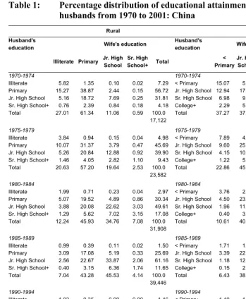
The marginal percentages distributions in Table 1 illustrate the changes in educational attainment for husbands and wives in this study. In general, the educational distribution changed substantially for both women and men. By 2000, more than two-thirds of rural women and three-quarters of rural men graduated from high school, while a high school education was nearly universal for urban couples. The overall rising rate of educational attainment was driven primarily by a substantial increase in high school graduates and a decrease in the number of individuals with less than an elementary school education. In rural areas, the percentage of husbands graduating from junior high school grew from 32% to 67%, while the percentage of wives graduating from junior high school expanded from 11% to 58%. In urban areas, the percentage of individuals completing senior high school among men increased from 25% to 38%, whereas this percentage nearly doubled among women, reaching 40% in 2000. In contrast, the percentage of couples attaining a college degree increased only in urban areas, rising from 18% to 31% for men and from 6% to 24% for women in these areas. Overall, husbands have achieved higher levels of education than wives within each marriage cohort.

8_{There are nine educational categories in the 2000 Census, and five educational categories in the 2001}

DRHS. I collapse the nine categories into four, in order to make the data from the two surveys parallel.

9_{“Senior high school” includes “Senior high school” and “Vocational high school” in the 2000 Census.} 10_{I grouped “College,” “University” and “Graduate” in the 2000 Census into the single education category}

“College and Up,” which is equivalent to “College and Up” in the 2001 DRHS. Approximately 8 percent of the sampled women age 15 to 49 belong in this category in both the 2000 Census and the 2001 DRHS.

11_{I grouped “No schooling” and “Recognize few words” into the category “Illiterate” in the 2000 Census; this}

(13)

Table 1: Percentage distribution of educational attainment for wives and husbands from 1970 to 2001: China

Rural Urban

Husband's

education Wife's education

Husband's

Illiterate Primary Jr. High School Sr. High School+ Total < Primary Jr. High School Sr. High School College + Total

1970-1974 1970-1974

Illiterate 5.82 1.35 0.10 0.02 7.29 < Primary 15.07 5.02 1.13 0.11 21.34

Primary 15.27 38.87 2.44 0.15 56.72 Jr. High School 12.94 17.23 3.82 0.76 34.74

Jr. High School 5.16 18.72 7.69 0.25 31.81 Sr. High School 6.98 9.67 7.56 1.49 25.69

Sr. High School+ 0.76 2.39 0.84 0.18 4.18 College+ 2.29 5.73 6.02 4.18 18.23

Total 27.01 61.34 11.06 0.59 100.0 Total 37.27 37.65 18.54 6.53 100.0

17,122 4,499

1975-1979 1975-1979

Total 20.63 57.20 19.64 2.53 100.0 Total 22.86 45.49 22.99 8.67 100.0

23,582 6,969

1980-1984 1980-1984

Total 12.24 45.93 34.76 7.08 100.0 Total 10.61 40.33 40.46 8.60 100.0

31,908 12,580

1985-1989 1985-1989

Total 7.04 43.28 45.53 4.14 100.0 Total 6.43 38.95 40.05 14.58 100.0

39,446 13,008

1990-1994 1990-1994

Total 5.86 42.75 48.44 2.96 100.0 Total 5.59 39.82 35.03 19.56 100.0

33,543 11,074

1995-2001 1995-2001

Total 4.24 33.38 57.77 4.61 100.0 Total 2.63 33.85 39.36 24.17 100.0

(14)

4. Log-linear models

This study uses log-linear models to analyze contingency tables in order to describe changes in patterns of educational assortative mating. Log-linear models provide estimates of the changing association between couples’ educational characteristics, controlling for shifts in their marginal distributions (Schwartz and Mare 2005). Homogamy models measure general trends in educational homogamy and crossing models reveal which educational differences between prospective spouses are serious barriers to intermarriage and which are relatively permeable (Mare 1991). I produced a contingency table with 192 cells (6×4×4×2) by cross-tabulating husbands’ education with wives’ education for the six marriage cohorts and two data sources. Each cell represents the number of first marriages between individuals with specific levels of education within a given marriage cohort and data source. The diagonal cells in the contingency table represent the homogamous marriages, while the off-diagonal cells represent the heterogamous marriages.

In order to estimate the log-linear models, I started with a baseline model, allowing three-way interactions among couples’ education by marriage cohort and data source:

HWD ijl WCD jkl HCD ikl WD jl HD il HW ij WC jk HC ik D l C k W j H i ijkl

F =β0+β +β +β +β +β +β +β +β +β +β +β +β log

ijkl

F

0

where is the expected frequency for cell ijkl in the contingency table; H, W, C, and D are the variables;12_and_i_,_j_,_k_{, and}_l_{are the categories within the variables}_H_,_W_,_C_,

and D. β is the grand mean of the natural log of the expected frequencies; , , , and are the main effects of husband’s education, wife’s education, cohort, and data source, respectively. and are the interactions between marriage cohorts and husband’s and wife’s education, respectively. and are the interactions between data source and husband’s and wife’s education. is the interaction between couples’ education and data source.

H i β W j β D l β HC β WD jl β HWD ijl β C k β ik β WC jk β HD il

In order to model the trends in educational homogamy, I added a homogamy parameter to the baseline model. This homogamy parameter is a 4×4 matrix with “1” in the diagonal cells and “0” in all other cells. Larger values in homogamy parameters

12_H_{: Husband’s education,}_i_=1-4;_W_{: Wife’s education,}_j_=1-4;_C_{: Marriage cohorts,}_k_=1-6;_D_{: Data sources,}

(15)

indicate that couples are more likely to marry those with similar levels of educational attainment. CO O HWD ijl WCD jkl HCD ikl WD jl HD il HW ij WC jk HC ik D l C k W j H i ijkl F β β β β β β β β β β β β β β + + + + + + + + + + + + + = 0 log (1) CO O β λ where allows the homogamy parameter to vary by cohort.

I specified crossing odds models in accordance with the clear applications of crossing odds models in Mare (1991) and Schwartz and Mare (2005). A series of crossing parameters were then added to the baseline model.

CX kp HWD ijl WCD jkl HCD ikl WD jl HD il HW ij WC jk HC ik D l C k W j H i ijkl F β β β β β β β β β β β β β β + + + + + + + + + + + + + = 0 log (2)

where X represents the crossing parameters, and represents the odds of crossing educational barriers.

CX kp

β

The odds of crossing the several barriers between men and women from different educational strata (i.e., marrying across groups) are a function of the β parameters (Mare 1991). Controlling for the marginal distribution of spouses’ education, the odds that a marriage observed in cohort k crosses barrier p is . Table 2 presents the contribution of each of these odds of intermarriage to the expected number of marriages. The crossing parameters indicate that couples with a greater distance between education levels have more barriers to cross. The estimated change in crossing parameters may provide evidence for variations in the rigidity of barriers across educational distribution over time.

)

exp( CX

kp X p

kp = β +β

Table 2: Parameters for crossings effects on educational assortative marriage

Husband's education Wife's education

Illiterate Elementary Junior high school Senior high school+

Illiterate 1 λ2 λ2λ3 λ2λ3λ4

Elementary λ2 λ λ3λ4

3 2λ

λ λ₄

4

3λ λ

1 3

Junior high school λ3 1

Senior high school+ λ2λ λ3λ4 4 1

(16)

5. Results

In this section, I first present a descriptive analysis of the trends in educational homogamy and heterogamy. I then describe the model selection process, and finally I summarize the estimated trends in educational homogamy and intermarriages yielded from the best fit models.

5.1 Trends in educational assortative marriage

5.1.1 Homogamous marriages and the rural-urban division

Figure 3 shows the changes in the percentage of educational assortative marriages for Chinese women age 15 to 49 married between 1970 and 2001.13_{The percentage of all}

marriages that were homogamous marriages first dropped and then climbed gradually between the 1980-1984 cohort and the 1995-2001 cohort. Among couples married in 1970-1974, 50.2% of wives shared the same level of educational attainment as their husbands. This percentage decreased to 49.2% for couples married between 1980 and 1984. Yet, the percentage of couples with the same years of schooling increased monotonically from 50% to 65% between the 1985-1989 marriage cohort and the 1995-2000 cohort. In short, at the national level there has been an overall 15-point increase in the percentage of educational homogamy among these six marriage cohorts from 1970 to 2000.

Panel B in Figure 3 illustrates the ways in which homogamy trends differed in urban and rural areas during this time period. The pattern of homogamy in rural areas has three distinctive features. First, the percentage of homogamous marriages among the rural sample of wives declined from 54% to 47% between 1970 and 1980, while the percentage among the urban sample increased from 44% to 54%. These contrasting trends for rural and urban wives offset each other, which explain the relatively stable trend at the national level. Second, between 1980 and 2001 the increases in the homogamy rate among wives in the rural sample were around four points larger than the increases for those in urban sample. Third, more than 80% of homogamous marriages in rural areas are between couples with less than a senior high school education, compared to less than 20% in urban areas. In addition, in rural areas the largest increase in homogamy rates was the six-fold increase in homogamous marriages

(17)

between junior high school graduates, while the largest increase in the urban sample was marriages among high school and college graduates. In short, the trends in homogamous marriage for the rural sample have distinctively different features from the patterns for the urban sample.

5.1.2 Heterogamous marriages and the rural-urban division

Panel A of Figure 3 illustrates the decreasing percentage of hypergamous marriages (i.e., wives marrying husbands with more education) among total marriages from 1970 to 2001. Among all marriages from the early 1970s, 45% of wives married husbands with higher levels of education, yet only 24% of wives followed this pattern in the late 1990s. Although the percentage of wives marrying husbands with lower levels of education continued to rise after the early 1980s, the increase was not sufficient to counteract the dropping heterogamous marriage rates caused by fewer wives marrying husbands with a higher education level.

Using the number of educational barriers crossed to investigate the changes in the percentage of heterogamous marriages, Panel A of Figure 4 provides additional evidence of a rising trend in educational homogamy. Compared to the trends described above, all intermarriages crossing any educational barriers showed a similar decline since the early 1980s. In particular, the percentage of intermarriages crossing one educational category, which accounted for 90% of the heterogamous marriages, declined from 40% to 30%. In addition, very few people with postsecondary education crossed three educational barriers and married an illiterate person.

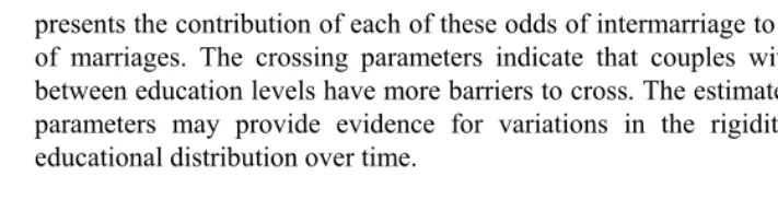
Panel B and C of Figure 4 reveal rural-urban differences in the timing and degree of intermarriage decreases. The decline in the percentage of heterogamy in urban areas started in the early 1970s—around a decade earlier than in rural areas. Further, the decline in the percentage intermarriages was larger in urban areas than rural areas. In urban areas, the predominant type of intermarriages starting in the early 1970s was marriages between elementary and junior high school graduates; these marriages experienced the largest drop, declining from 48% to 8%. In contrast, in rural areas, the largest percentage drop, from 40% to 8%, took place among marriages formed between illiterate respondents and elementary school graduates. In short, the decline in the rate of heterogamy occurred earlier and was greater in urban areas than in rural areas. Overall, the rural-urban division in the decline of intermarriages is consistent with the different patterns of educational homogamy between rural and urban areas.

(18)

than rural areas. However, the average educational attainment of both men and women increased in this time period, therefore the patterns described above may be partially due to changes in the educational levels of potential partners in the marriage pool (Mare 1991). Therefore, I use log-linear models to estimate the trends in educational homogamy in China from 1970 to 2000; these models reduce the distortion introduced by changes in the marginal distribution.

5.2 Selection of models

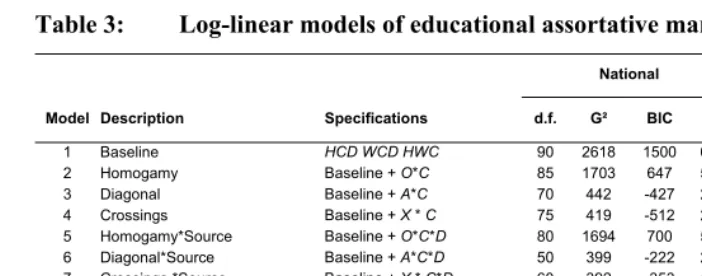
Table 3 reports the deviance G² (-2*log-likelihood) and Bayesian Information Criteria (BIC) statistics for log-linear models of the trends in assortative marriage rates between 1970 and 2000 for national, rural and urban samples. Models with the smallest G² and most negative BIC fit the pooled data most closely. Because the model fit statistics for the rural and urban samples resemble those for the national sample, I present the model selection process for the national sample.

(19)

Figure 3: Changes in the percentage of educational assortative marriages for women age 15-49: China, 1970-2001

Panel A. Percentage of homogamous and heterogamous marriages at the national level

0.0 10.0 20.0 30.0 40.0 50.0 60.0 70.0 80.0

P

erc

ent

(%

)

1970-19 74

1975-1979 1980-1984

1985-198 9

1990-1994 1995-20 01

Marriage Cohort

Percent homogamy Percent hypergamy

Percent hypogamy

Panel B. Percentage of homogamous marriages at the rural and urban sample

40.0 45.0 50.0 55.0 60.0 65.0 70.0

P

erc

en

t (%)

1970-1974

1975-1979

1980-1984

1985-1989

1990-1994

1995-2001

Marriage Cohort

Urban Rural

(20)

Figure 4: Percentage of heterogamous marriages crossing educational levels for women age 15-49: China, 1970-2001

Panel A. National sample

0.0 10.0 20.0 30.0 40.0 50.0 Perc ent (%) 197 0-1974 1975 -197 9 1980 -198 4 1985 -198 9 1990 -199 4 1995 -200 1 Marriage Cohort

Crossing one Crossing two Crossing three

Panel B. Urban sample

0.0 10.0 20.0 30.0 40.0 50.0 60.0 70.0 80.0 Pe rce n t (%) 197 0-1974 19 75-1979 1980-1984 1985-1989 1990 -1994 199 5-2001 Marriage Cohort

Jr.High/<Elementary Sr.High/Jr.High College+/Sr.High

(21)

Figure 4: (Continued) Panel C. Rural sample

0.0 10.0 20.0 30.0 40.0 50.0 60.0 70.0 80.0

P

e

rcent (%

)

19 70-1974

19 75-1979

1980 -198

4

19 85-1989

19 90-1994

19 95-2001

Marriage Cohort

Elementary/Illiterate Jr.High/Elementary Sr.High+/Jr.High

In order to test the hypothesized time-varying patterns in the permeability of educational barriers, I add crossing parameters for three educational barriers to the baseline model in Model 4, allowing the crossing parameters to be cohort-specific. The crossing model (Model 4) fits the data better than Model 3, with a significant reduction in G² (G²[3]- G²[4]=23. d.f.=-5) and BIC (BIC[3]-BIC[4] =85). Therefore, the time-varying crossing models capture variations in patterns of educational assortative mating well. In addition, Models 5-7 test the hypothesis that the association and crossing parameters vary by data source. Judging by the criteria of G² and BIC, these models fail to generate a better fit than Models 2-4. These results suggest that the estimated association and crossing parameters do not vary by data source. Therefore, I present the remaining results using pooled data.14

(22)

Table 3: Log-linear models of educational assortative marriages (N=235,075)

National Rural Urban

Model Description Specifications d.f. G² BIC G² BIC G² BIC

1 Baseline HCD WCD HWC 90 2618 1500 672 -414 503 -487

2 Homogamy Baseline + O*C 85 1703 647 529 -497 389 -545

3 Diagonal Baseline + A*C 70 442 -427 291 -553 265 -504

4 Crossings Baseline + X * C 75 419 -512 239 -667 176 -648

5 Homogamy*Source Baseline + O*C*D 80 1694 700 506 -459 386 -493

6 Diagonal*Source Baseline + A*C*D 50 399 -222 249 -354 249 -311

7 Crossings *Source Baseline + X * C*D 60 392 -353 188 -536 159 -500

8 Crossings, Homogamy Baseline + X*C O*C 70 118 -751 109 -744 60 -710

9 Crossings, Diagonal Baseline + X*C A*C 65 103 -704 90 -694 57 -657

10 Crossings, Homogamy,

Hypergamy Baseline + X*C O*C P*C 65 99 -708 95 -689 55 -660

11 Crossings, Diagonal, HypergamyBaseline + X*C A*C P*C 60 80 -665 85 -639 53 -607

Note: H=Husband’s education (1-4), W=Wife’s education (1-4), C=Cohort (1-6), D=Data source (0,1), O=Homogamy (0,1),

A=Diagonal (1-4), X=Crossing parameters (1-3), P=Hypergamy (0,1).

Models 8-11 relax the assumption that the homogamy, diagonal and hypergamy parameters are all time invariant in the crossing model. All of these models fit better than Model 4 with restrictions. Model 8 (crossing with homogamy) fits the data most closely, as indicated by the most negative BIC (BIC[4]-BIC[8] =239, d.f.=5). These results suggest that: (1) patterns of educational assortative marriage changed among the six marriage cohorts and (2) temporal variations were captured by changes in crossing parameters and homogamy parameters.

5.3 Results of Log-linear models

5.3.1 Estimated trends in educational homogamy at the national level

(23)

1980s is consistent with previous results reported by Raymo and Xie (2000) and Smits, Ultee and Lammers (2000).

In contrast, the rising homogamous marriage rates after the mid-1980s are a new phenomenon. The odds of homogamy shifted direction following the early 1980s. Indeed, a dramatic increase in the odds of educational homogamy took place between 1980 and 1994. The odds of homogamy climbed from 6.0 for the 1980-1984 cohort to 9.0 for the 1995-2001 marriage cohort. These results suggest that the association between spouses’ educational attainment has strengthened between 1980 and 2001. Overall, the estimated increasing national-level rate of educational homogamy between the 1980s and 1990s is consistent with studies based on the 1990 China Census and other Surveys (Esteve and McCaa 2008; Song 2009), despite different degrees of homogamy.

To further validate the trends found above, I calculated the odds ratios of marrying a partner with a similar education level, relative to crossing into the adjacent category and entering a heterogamous marriage for members of all marriage cohorts in national, urban and rural samples, using the methods illustrated in Smits and Park (2009). In Appendix 2 I reported the odds ratios based upon the 2*2 contingency table. At the national level, the odds of forming educationally homogamous marriages relative to intermarriages increased across the six marriage cohorts for any educational strata despite declines or fluctuations before 1980. The trends for the odds ratios in rural and urban areas essentially resembled the increasing homogamy trends estimated from the log-linear model in Figure 5. In short, both the log-linear modeling approach and the 2*2 contingency table method reveal rising educational homogamy between 1980 and 2000 in China.15

5.3.2 The rural-urban division in educational homogamy

Although the results for the rural sample resemble the national-level decline and increase in educational homogamy, the urban sample shows a distinct pattern with regard to both the degree and the timing of changes. Compared to the same cohort in the rural sample, the estimated odds of educational homogamy were 1.7 points lower for the 1970-1974 marriage cohort of the urban sample. Yet, the rural-urban

(24)

discrepancy in the odds of educational homogamy began to diminish among the 1995-2001 cohorts. There were also rural-urban differences in timing; the estimated odds of educational homogamy started to increase approximately ten years earlier in the urban sample than in the rural sample. The resemblance in education among urban couples began to increase in the late 1970s, while rural couples were increasingly more likely to marry within their own educational categories only after the mid-1980s.

The current results indicating increasing educational homogamy in urban areas after the 1970s are consistent with results reported in a study of 20 cities in China (Song 2009). Using data from “The State and Life Chances in China from 1949-94,” Song (2009) found the rate of educational homogamy was higher among the 1977-1994 marriage cohorts than among the 1966-1976 cohorts. Using refined measures of marriage cohorts, this study not only identifies the timing and patterns of increasing homogamy between 1970 and 1990, but also reveals slower growth in the late 1990s in urban areas. Further, this study is the first to show increasing spousal resemblance in rural areas after the early 1980s. In short, the current results—showing rising levels of educational homogamy in both urban and rural areas—support the first hypothesis, which states that educational expansion, the increasing economic value of education, and the increasingly common practice of delaying marriage have all led to important changes in marriage patterns. Greater degrees of spousal resemblance in China in the late 1990s also indicate higher levels of social closure across educational strata.

(25)

Figure 5: Estimated odds of educational homogamy relative to heterogamy for women age 15-49: China, 1970-2001

6.0 6.5 7.0 7.5 8.0 8.5 9.0 9.5 10.0

odds

of hom

ogam

y

1970-1974 1975-1979 1980-1984 1985-1989 1990-1994 1995-2001

Marriage Cohorts

National Urban Rural

5.3.3 Estimated trends in educational heterogamy

The crossing odds represent couples’ hesitation to enter into intermarriages. I summarize the odds of crossing any educational barriers for respondents with all levels of education in Table 4. The crossing models show that the odds of intermarriage declined across all levels of the educational distribution after the early 1980s, which confirms the increasing educational homogamy rate estimated above. The parallel declines of the crossing odds indicate that, compared to those who married in the 1970s, couples who married in the 1990s were less likely to cross educational barriers and more likely to marry within their educational categories. Because more than 80% of intermarriages crossed one educational barrier, I present the parameter estimates for crossing one educational barrier for women age 15 to 49 in China in Figure 6.

(26)

roughly similar across the entire educational distribution. For each group, the odds of intermarriages were cut in half between 1985 and 1995. For high school or college graduates, the odds of marrying a junior high school graduate declined from 0.5 to 0.2. In short, couples married between 1980 and 1994 experienced the most remarkable reduction in the probability of marrying a partner with less education. As more than two-thirds of respondents graduated from high school in the late 1990s, these declining rates of intermarriage indicate that the once permeable barriers became rigid. Finally, the results reveal that high school graduates, who had the highest odds of heterogamy in both rural and urban samples, experienced a larger drop in the odds of intermarriage than those located either at the top or at the bottom of the educational distribution between the early 1980s and late 1990s. Overall, this trend of declining odds of educational heterogamy is in line with the increasing odds of homogamy. In short, the fact that the largest drop in the odds of marrying a partner with less education occurs for high school graduates confirms my second hypothesis. These findings suggest that the permeability of barriers to secondary education in the marriage market was also lowered in the 1990s.

Panels B and C of Figure 6 show that urban couples differed significantly from rural couples in the odds of marrying a partner with less education. Differences lay in the magnitude and timing of the decline, despite parallel drops in the crossing odds. First, the rate of marrying a partner with less education was lower in urban areas than in rural areas across the entire educational distribution, indicating a more rigid urban marriage market. In particular, the barriers to marrying highly educated respondents were less permeable in urban areas than in rural areas. For example, among the 1970-1974 cohort, a senior high school graduate in an urban area was 0.6 times less likely to marry a junior high school graduate than to marry a classmate; however, in rural areas high school graduates in the 1970-1974 cohort were 0.4 times less likely to marry a junior high graduate. This ratio declined to from 1.5 to 1 for the 1995-2001 cohort. In addition, the odds of marrying a partner with less education among college graduates in urban areas remained below 0.1 between 1970 and 2001, suggesting that college education may be the most difficult barrier to cross.

(27)

Figure 6: Estimated odds of crossing one educational barrier, relative to homogamy for women age 15-49: China, 1970-2001

Panel A: National Sample

0.0 0.1 0.2 0.3 0.4 0.5 0.6 0.7 0.8 0.9 1.0

Odds of C

rossing

1970-1974 1975-1979 1980-1984 1985-1989 1990-1994 1995-2001

Marriage Cohorts

Panel B: Urban Sample

0.0 0.1 0.2 0.3 0.4 0.5 0.6 0.7 0.8 0.9 1.0

O

dds

of Cr

os

si

ng

1970-1974 1975-1979 1980-1984 1985-1989 1990-1994 1995-2001

Marriage Cohorts

Jr.High/<Elementary Sr.High/Jr.High College+/Sr.High

(28)

Figure 6: (Continued) Panel C: Rural Sample

0.0 0.1 0.2 0.3 0.4 0.5 0.6 0.7 0.8 0.9 1.0

Odds

of

C

ros

si

ng

1970-1974 1975-1979 1980-1984 1985-1989 1990-1994 1995-2001

Marriage Cohorts

Considering the fact that the overall odds of educational homogamy increased after the early 1980s, the decline in odds of intermarriages crossing one educational barrier further indicate that people with high school or college education may increasingly marry within their own educational category, and there are fewer chances for people with low education to marry a partner with a higher level of education. Since intermarriages crossing one educational barrier account for nearly 80% of the total intermarriages and two-thirds of respondents had secondary and postsecondary education, the greatest drop in the odds of intermarriages among these high school graduates between 1985 and 1994 may leave a large number of poorly educated people behind in the marriage market.

(29)

among college graduates than among other educational groups. These findings also indicate that it is increasingly difficult for the poorly educated to move up the social strata through marriage.

In summary, my investigation of educational homogamy and intermarriage yields consistent findings that the odds of educational homogamy increased between 1980 and 2000; however, the odds of intermarriage across educational barriers varied across the educational distribution and by rural/urban status. The generally decreasing odds of crossing any educational barriers for all educational categories provide strong evidence that the social distance between groups has strengthened between 1984 and 2001 in China.

Table 4: Estimated odds of crossing educational barriers for women age 15-49: China, 1970-2001

Rural Urban

Husband's

education Wife’s education

Husband's

Illiterate Elementary Junior high school

< Elementary

Junior high school

Senior high school

1970-1974 1970-1974

Elementary 0.468 Junior high school 0.114

Junior high school 0.196 0.419 Senior high school 0.063 0.554

Senior high school+ 0.131 0.279 0.667 College and up 0.014 0.119 0.215

1975-1979 1975-1979

1980-1984 1980-1984

1985-1989 1985-1989

1990-1994 1990-1994

1995-2001 1995-2001

(30)

5.4 Explanations of rising educational homogamy trends

One possible explanation of rising rates of educational homogamy in China after the 1980s is that economic returns on education increased between 1970 and 2000. Increasing homogamy at the national level coincided with the increasing economic value placed on education during the market transition. Wider income inequalities across educational strata in urban areas echoed greater degrees of social closure in the marriage market.

At the national level, returns on schooling increased rapidly between the late 1970s and the late 1980s, and then accelerated even more in the 1990s (Fleisher, Sabirianova and Wang 2005). The high yields of education may have increased people’s motivation to find highly educated partners. Most importantly, the education premium became larger for high school and college graduates. Moderate estimates showed that the economic returns on college education, relative to high school, rose from 4.9% in 1988 to 15.0% in 1995 (Knight and Song 2003). In addition to direct economic rewards, a college degree was crucial to provide access to prestigious occupations and promotional opportunities (Zhao and Zhou 2007). In short, highly educated Chinese individuals may be eager to maintain and increase their social status by marrying an equally educated person, resulting in higher levels of educational homogamy.

The distinct patterns of educational homogamy for rural and urban areas echoed the lasting rural-urban division in education rewards in contemporary China. First, the economic returns on education were higher in urban areas than in rural areas due to a unique occupational structure and reward system. After the 1979 reform, the burgeoning private sector rewarded the highly educated in urban areas (Li 2003) and one additional year of schooling was, on average, associated with a 10.2% increase in wages in 2000 (Zhang et al. 2005). Schooling, however, did not enhance the productivity of farm workers and therefore did not yield direct economic value in rural China (Zhao 1999). Studies showed that the economic returns on schooling in farming areas only rose to a positive return of about 3% for household farming in 1990 (Li and Zhang 1998). In addition, the average return on a year of education was 4.3% among rural local wage earners, whereas it was 7.8% among all migrants in 2000 (De Brauw and Rozelle 2008). In short, given that urban areas produce higher economic returns on education, the highly educated in these areas are more likely to marry homogamously than to marry a partner with less education.

(31)

township-owned enterprises and migration offered opportunities to earn income and increased incentives to invest in education (Yang 1997; Zhao 1999). Thus, the later increases in schooling returns in rural areas may be associated with later increases in educational homogamy.

Third, income inequality across educational strata became wider in urban areas than in rural areas. In urban areas, the income gaps between college graduates and those with elementary school education or illiterates nearly doubled after 1979 (Zhou 2002). In contrast, in the rural sector, economic returns on secondary education, relative to elementary education were 11.2% in 1991, and the income gap between elementary school graduates and illiterate respondents was even smaller (Wei, et al. 1999). Thus, given the greater rewards experienced by highly educated individuals and the presence of wider income gaps across the educational strata in urban areas, the chances of entering intermarriages across educational barriers are slimmer in these areas, compared to rural areas, and thus the barriers to marrying a partner with more education experienced by the poorly educated are more difficult to overcome.

In summary, increasing economic returns on senior high school and college education may be associated with a greater degree of educational homogamy in China from 1970 to 2000. As higher levels of education promised economic prosperity and security, and the income gaps between the highly educated and the poorly educated became wider, the highly educated had more incentive to maintain or increase their social status by marrying within their own educational category. As the income gaps across the educational strata were larger in urban areas than in rural areas, the estimated trends in intermarriage revealed a lower degree of heterogamous marriages and less permeable educational barriers in the urban marriage market.

6. Summary and conclusion

(32)

identifying increasing homogamy in China after the early 1980s. Furthermore, this study finds that increasing spousal resemblance occurred a decade earlier and at a higher level in urban areas compared to rural areas. Urban areas showed consistently increasing rates while rural area rates declined before the 1980s. In short, this study is the first to report the distinct rural-urban division of educational homogamy in China during the period from 1970 to 2000.

In order to determine how patterns of intermarriage varied across the educational distribution, I used crossing models to estimate differences in the odds of crossing barriers for people with different levels of education. Results showed that more intermarriages took place between people with middle levels of education than people both at the top and bottom. In addition, a greater drop in the odds of intermarriage occurred among people with middle levels of education, which indicates that people at the bottom of the educational strata increasingly have fewer chances to marry a partner with a higher level of education. Second, consistent decreases in the odds of crossing any barrier for college and senior high school graduates suggest growing social closure among the highly educated because they are less likely to marry outside their own educational group.

In short, I demonstrate that the national-level educational homogamy rates increased substantially between 1980 and 2000, as China experienced booming economic growth and a market transition. The findings are consistent with the status attainment hypothesis. During the unprecedented process of social change, the burgeoning number of homogamous marriages among highly educated individuals suggests that people greatly value education in spousal selection. The increasing educational homogamy rates parallel rising economic returns on education, since China experienced a sweeping market transition. As the earning gap between highly educated individuals and poorly educated individuals widened, highly educated individuals increasingly married within their own group to maintain their social status. These respondents were less likely to cross any educational barriers and more likely to avoid downward mobility. As a result, poorly educated people have much lower chances of achieving higher social status through marriage. The much wider earning gaps across the educational strata in urban areas provide plausible explanations for the greater degrees of social closure in urban areas.

(33)

capital increase, households formed by people with lower educational levels may be more disadvantaged, because they lack access to both education and political capital. As a result, the concentration of marriages within lower education categories may generate continuous inequalities in this generation as well as in future generations in China.

Future studies are needed in three areas. First, studies employing a life course approach and longitudinal studies of individual marital choices will help researchers identify key factors influencing marriage patterns (Blossfeld 2009). Second, a two-sided choice model should be employed to analyze the actual mate selection process which includes preferences and potential partners of both husbands and wives. This method will allow a more nuanced understanding of the critical role of education in the marriage market. Third, a study of marriage patterns among migrant workers is necessary as the rural-to-urban migration movement in the 1990s brought substantial changes to the cultural and economic value of education in rural China.

7. Acknowledgements

(34)

References

Bian, Y. and Logan, J.R. (1996). Market transition and the persistence of power: The changing stratification system in urban China. American Sociological Review 61(5): 739-578. doi:10.2307/2096451.

Bian, Y. (2002). Chinese social stratification and social mobility. Annual Review of Sociology 28: 91-116. doi:10.1146/annurev.soc.28.110601.140823.

Blossfeld, H. (2009). Educational assortative marriage in comparative perspective. Annual Review of Sociology 35(1): 513-530. doi:10.1146/annurev-soc-070308-115913.

De Brauw, A. and Rozelle, S. (2008). Reconciling the returns to education in off-farm wage employment in rural China. Review of Development Economics 12(1): 57-71. doi:10.1111/j.1467-9361.2007.00376.x.

Deng, Z. and Treiman, D.J. (1997). The impact of the cultural revolution on trends in educational attainment in the People's Republic of China. The American Journal of Sociology 103(2): 391-428. doi:10.1086/231212.

Diamant, N.J. (2000). Re-examining the impact of the 1950 marriage law: State improvisation, local initiative and rural family change. The China Quarterly (161): 172-198. doi:10.1017/S0305741000003982.

Ermisch, J., Francesconi, M., and Siedler, T. (2006). Intergenerational mobility and marital sorting. The Economic Journal 116(513): 659-679. doi:10.1111/j.1468-0297.2006.01105.x.

Esteve, A. and McCaa, R. (2008). Assortativemating patterns in the developing world. Paper presented at the 2009 IUSSP Seminar on Changing Transitions to Marriage, New Delhi, September 10-12, 2008.

Fan, C. and Huang, Y. (1998). Waves of rural brides: female marriage migration in China. Annals of the Association of American Geographers 88(2): 227-251.

doi:10.1111/1467-8306.00092.

Fernandez, R., Guner, N., and Knowles, J. (2005). Love and money: A theoretical and empirical analysis of household sorting and inequality. The Quarterly Journal of Economics 120(1): 273-344. doi:10.1162/0033553053327498.

(35)

Goodkind, D. and Branch, E. (2006). Marriage squeeze in China: historical legacies, surprising findings. Paper presented at the 2006 Annual Meeting of the Population Association of America, Los Angeles, March 30-April 1, 2006. Hannum, E. (1999). Political change and the urban-rural gap in basic education in

China, 1949-1990. Comparative Education Review 43(2): 193-211.

doi:10.1086/447554.

Hannum, E., Wang, M. and Adams, J. (2008). Urban-rural disparities in access to primary and secondary education under market reform. In: Whyte, M.K. (ed.). One country, two societies? Rural-urban inequality in contemporary China. Cambridge: Harvard University Press.

Hauser, S.M. and Xie, Y. (2005). Temporal and regional variation in earnings inequality: Urban china in transition between 1988 and 1995. Social Science Research 34(1): 44-79. doi:10.1016/j.ssresearch.2003.12.002.

International Monetary Fund (2000). The World Economic Outlook (WEO) database [electronic resource]. Washington, D.C.: International Monetary Fund.

http://www.imf.org/external/pubs/ft/weo.

Kalmijn, M. (1991). Status homogamy in the United States. The American Journal of Sociology 97(2): 496-523. doi:10.1086/229786.

Kalmijn, M. (1998). Intermarriage and homogamy: Causes, patterns, trends. Annual Review of Sociology 24: 395. doi:10.1146/annurev.soc.24.1.395.

Knight, J. and Song, L. (2003). Increasing wage inequality in China: Extent, elements and evaluation. Economics of Transition 4: 597-619. doi:10.1111/j.0967-0750.2003.00168.x.

Lewis, S.K. and Oppenheimer, V.K. (2000). Educational assortative mating across marriage markets: Non-hispanic whites in the United States. Demography 37(1): 29-40. doi:10.2307/2648094.

Li, B. and Walder, A.G. (2001). Career advancement as party patronage: Sponsored mobility into the Chinese administrative elite, 1949-1996. The American Journal of Sociology 106(5): 1371-1408. doi:10.1086/320816.

Li, H. (2003). Economic transition and returns to education in China. Economics of Educational Review 22(3): 317-328. doi:10.1016/S0272-7757(02)00056-0. Li, T. and Zhang, J. (1998). Returns to education under collective and household

farming in China. Journal of Development Economics 56(2): 307-335.

doi:10.1016/S0304-3878(98)00068-6.

(36)

National Bureau of Statistics of China (2000). China Population Census. Beijing: National Bureau of Statistics of China.

Nee, V. and Matthews, R. (1996). Market transition and societal transformation in reforming state socialism. Annual Review of Sociology 22: 401-435.

doi:10.1146/annurev.soc.22.1.401.

Nee, V. (1991). Social inequalities in reforming state socialism: Between redistribution and markets in china. American Sociological Review 56(3): 267-282.

doi:10.2307/2096103.

Nee, V. (1989). A theory of market transition: From redistribution to markets in state socialism. American Sociological Review 54(5): 663-681. doi:10.2307/2117747. Pochagina, O. (2004). Chinese youth: Attitude toward family and marriage. Far

Eastern Affairs 32(1): 133-149.

Qian, Y. (2000). The process of China's market transition (1978-1998): The evolutionary, historical, and comparative perspectives. Journal of Institutional and Theoretical Economics 156(1): 151.

Qian, Z. and Preston, S.H. (1993). Changes in American marriage, 1972 to 1987: Availability and forces of attraction by age and education. American Sociological Review 58(4): 482-495. doi:10.2307/2096072.

Qian, Z. (1998). Changes in assortative mating: The impact of age and education, 1970-1990. Demography 35(3): 279-292. doi:10.2307/3004036.

Raymo, J.M. and Xie, Y. (2000). Temporal and regional variation in the strength of educational homogamy. American Sociological Review 65(5): 773-781.

doi:10.2307/2657546.

Schwartz, C.R. and Mare, R.D. (2005). Trends in educational assortative marriage from 1940 to 2003. Demography 42(4): 621-646. doi:10.1353/dem.2005.0036. Schwartz, C.R. and Mare, R.D. (2003). The effects of marriage, marital dissolution, and

educational upgrading on educational assortative mating. [unpublished manuscript] Los Angeles:California Center of Population Research.

Shu, X. and Bian, Y. (2003). Market transition and gender gap in earnings in urban China. Social Forces 81(4): 1107-1145. doi:10.1353/sof.2003.0070.

Shu, X. (2004). Education and gender egalitarianism: The case of China. Sociology of Education 77(4): 311-336. doi:10.1177/003804070407700403.

(37)

Smits, J., Ultee, W., and Lammers, J. (2000). Reply to Raymo and Xie: More or less educational homogamy? A test of different versions of modernization theory using cross-temporal evidence for 60 countries. American Sociological Review 65(5): 781-788. doi:10.2307/2657547.

Smits, J. (2003). Social closure among the higher educated: Trends in educational homogamy in 55 countries. Social Science Research 32(2): 251-277.

doi:10.1016/S0049-089X(02)00049-2.

Smits, J. and Park, H. (2009). Five decades of educational assortative mating in ten East Asian societies. Social Forces 88(1): 227-255. doi:10.1353/sof.0.0241.

Song, L. (2009). The effect of the cultural revolution on educational homogamy in urban China. Social Forces 88(1): 257. doi:10.1353/sof.0.0246.

State Fertility Planning Commission of China (2001). Chinese Demographic Reproductive Health Survey. Beijing: State Fertility Planning Commission of China.

Walder, A.G. (1996). Markets and inequality in transitional economies: Toward testable theories. The American Journal of Sociology 101(4): 1060. doi:10.1086/230789. Walder, A.G. (2002). Markets and income inequality in rural china: Political advantage

in an expanding economy. American Sociological Review 67(2): 231-253.

doi:10.2307/3088894.

Wang, F. (2005). Organizing through division and exclusion: China’s hukou system. Stanford: Stanford University Press.

Wei, X., Tsang, M.C., Xu, W., and Chen, L. (1999). Education and earnings in rural China. Education Economics 7(2): 167-187. doi:10.1080/09645299900000014. Wu, X. and Treiman, D.J. (2004). The household registration system and social

stratification in China: 1955-1996. Demography 41(2): 363-384.

doi:10.1353/dem.2004.0010.

Xia, Y. and Zhou, Z. (2003). The transition of courtship, mate selection and marriage in China. In: Hamon, R. and Ingoldsby, B. (eds.). Mate Selection Across Cultures. Thousand Oaks: Sage Publications, Inc. 231-246.

Xie, Y. and Hannum, E. (1996). Regional variation in earnings inequality in reform-era urban China. The American Journal of Sociology 101(4): 950-992.

doi:10.1086/230785.

Xu, X., Ji, J., and Tung, Y. (2000). Social and political assortative mating in urban

China. Journal of Family Issues 21(1): 47-77.

(38)

Xu, X. and Whyte, M. (1990). Love matches and arranged marriages: A Chinese replication. Journal of Marriage and the Family 52(3): 709-722.

doi:10.2307/352936.

Yang, D.T. (1997). Education and off-farm work. Economic Development and Cultural Change 45(3): 613-632. doi:10.1086/452293.

Zhang, J., Liu, P., and Yung, L. (2007). The Cultural Revolution and returns to schooling in China: Estimates based on twins. Journal of Development Economics 84(2): 631-639. doi:10.1016/j.jdeveco.2006.12.006.

Zhang, J., Zhao, Y., Park, A., and Song, X. (2005). Economic returns to schooling in urban China, 1988 to 2001. Journal of Comparative Economics 33(4): 730.

doi:10.1016/j.jce.2005.05.008.

Zhao, Y. (1997). Labor migration and returns to rural education in China. American Journal of Agricultural Economics 79(4): 1278-1287. doi:10.2307/1244284. Zhao, Y. (1999). Labor migration and earnings differences: The case of rural China.

Economic Development and Cultural Change 47(4): 767-782.

doi:10.1086/452431.

Zhao, W. and Zhou, X. (2007). Returns to education in China’s transitional economy: Reassessment and reconceptualization. In: Hannum, E. and Park, A. (eds.). Education and Reform in China. Oxford: Routledge.

Zhou, X., Moen, P., and Tuma, N.B. (1998). Educational stratification in urban China: 1949-1994. Sociology of Education 71(3): 199-222. doi:10.2307/2673202. Zhou, X. (2000). Economic transformation and income inequality in urban China:

(39)

Appendix 1: Number of observations in pooled sample with six cohorts for women age 15-49 in China

Cohorts Rural Urban

Census Survey Census Survey Total

1970-1974 15,646 1,476 4,293 206 21,621

1975-1979 20,471 3,111 6,230 739 30,551

1980-1984 27,126 4,782 10,861 1,719 44,488 1985-1989 33,763 5,683 11,134 1,874 52,454 1990-1994 28,697 4,756 9,449 1,625 44,527 1995-2001 25,117 4,677 9,964 1,676 41,434

Total 150,820 24,485 51,931 7,839 235,075