Mathematics Interdisciplinary Research (MIR) publishes quality original research papers and survey articles in Interdisciplinary Mathematics that are of the highest possible quality. The editorial board of this journal comprises experts from around the world. The papers in the relationship between two different scientific disciplines are of high interest for MIR. The research papers and review articles are selected through a normal refereeing process by a member of editorial board. A paper acceptable for publication must contain non-trivial mathematics with clear applications to other parts of science and engineering. MIR motivates authors to publish significant research papers, which are of broad interests in Applications of Mathematics in Science. Two issues in one volume are published every year.
Aims and Scope: MIR contains research articles in the form of expository papers, original scientific article, short communications on important mathematical problems of basic sciences and letter to the editor. The submission of a paper implies that the author(s) assurance that it has not been copyrighted, published, or submitted for publication elsewhere. All accepted papers in MIR will be checked against plagiarism by iThenticate.
Preparation of Manuscripts: An abstract of 150 words or less and keywords clarifying the subject of the manuscripts are required. Authors should submit the paper via our online system at mir.kashanu.ac.ir. All correspondence has to be sent to the address [email protected].
The language of the journal is English. Authors who are less familiar with English language are advised to seek assistance from proficient scholars to prepare manuscripts that are grammatically and linguistically free from errors. Papers submitted for consideration for publication have to be prepared concisely and must not exceed 60 typewritten pages, (font 12, double spacing, including tables & graphs).
Photographs must be printed on contrasted glossy paper and have sharp outlines. Diagrams and figures should be submitted as original drawings. Figures and tables are to be numbered in the sequence in which they are cited in the manuscript. Every table and figure must have a caption that explains its content. Tables and diagrams are to be prepared in separate pages and placed at the end of the manuscript.
References to the literature should be numbered in square brackets in the order in which they appear in the text. A complete list of references should be presented in numerical order at the end of the manuscript. References to journals, books, proceedings and patents must be presented in accordance with the following examples:
Journals: I. Gutman, B. Zhou, B. Furtula, The Laplacian-energy like invariant is an energy like invarint, MATCH Commun. Math. Comput. Chem. 64(1) (2010) 85-96.
Book: A. A. Ungar, Beyond the Einstein Addition Law and its Gyroscopic Thomas Precession: The Theory of Gyrogroups and Gyrovector Spaces, Volume 117 of Fundamental Theories of Physics, Kluwer Academic Publishers Group, Dordrecht, 2001.
Book Chapter: T. Suksumran, The algebra of gyrogroups: Cayley’s theorem, Lagrange’s theorem and isomorphism theorems, in: Essays in Mathematics and its Applications: In Honor of Vladimir Arnold, T. M. Rassias, P. M. Pardalos (Eds.), Springer, New York, 2016.
Patents: H. S. Primack, Method of Stabilizing Polyvalent Metal Solutions, U.S. patent No. 4, 373, 104 (1983). Proofs and Reprints:
Editor-in-Chief:
Ali Reza Ashrafi
Department of Pure Mathematics, Faculty of Mathematical Sciences, University of Kashan, Kashan
87317-53153, I. R. Iran
E-mail: [email protected]
Director-in-Charge:
Majid Monemzadeh
Department of Particle Physics and Gravity, Faculty of Physics, University of Kashan, Kashan
87317-53153, I. R. Iran
E-mail: [email protected]
Executive Manager:
Fatemeh Koorepazan-Moftakhar
Department of Pure Mathematics, Faculty of Mathematical Sciences, University of Kashan, Kashan
87317-53153, I. R. Iran
E-mail: [email protected]
Language Editor:
Seyfollah Mosazadeh
Department of Pure Mathematics, Faculty of Mathematical Sciences, University of Kashan, Kashan
87317-53153, I. R. Iran
E-mail: [email protected]
Editorial Board
Ali Reza Ashrafi
University of Kashan, I. R. Iran
E-mail: [email protected]
Seyed Morteza Babamir
University of Kashan, I. R. Iran
E-mail: [email protected]
Alain Bretto
Universite de Caen, France
E-mail: [email protected]
Bijan Davvaz
Yazd University, I. R. Iran
E-mail: [email protected]
Mircea V. Diudea
Babes-Bolyai University, Romania
E-mail: [email protected]
Tomislav Došlić
University of Zagreb, Croatia
E-mail: [email protected]
Wiesław A. Dudek
Wrocław University of Technology, Poland
E-mail: [email protected]
Changiz Eslahchi
Shahid Beheshti University, I. R. Iran
E-mail: [email protected]
Gholam Hossein Fath
Tabar
University of Kashan, I. R. Iran
Mohammad Ali Iranmanesh
Yazd University, I. R. Iran
E-mail: [email protected]
Gyula O. H. Katona
Alfréd Rényi Institute of Mathematics, Hungary
E-mail: [email protected]
G. Ali Mansoori
University of Illinois at Chicago, USA
E-mail: [email protected]
Majid Monemzadeh
University of Kashan, I. R. Iran
E-mail: [email protected]
Sirous Moradi
Arak University, I. R. Iran
E-mail: [email protected]
Ottorino Ori
Actinum Chemical Research, Italy
E-mail: [email protected]
Abbas Saadatmandi
University of Kashan, I. R. Iran
E-mail: [email protected]
Ruggero Maria Santilli
The R. M. Santilli Foundation, USA
E-mail: [email protected]
Yongtang Shi
Nankai University, P. R. China
E-mail: [email protected]
Abraham A. Ungar
North Dakota State University, USA
E-mail: [email protected]
Hassan Yousefi-Azari
University of Tehran, I. R. Iran
E-mail: [email protected]
Janez Žerovnik
University of Ljubljana, Slovenia
E-mail: [email protected]
Editorial Office:
Department of Pure Mathematics, Faculty of Mathematical Sciences, University of Kashan, Ravand
Boulevard, Kashan 87317-53153, I. R. Iran
Volume 1, Issue 2, Summer 2016, Page 273-334
Contents
Pages
Motion of Particles under Pseudo-Deformation
Akhilesh Chandra Yadav
273
C-Class Functions and Remarks on Fixed Points of Weakly Compatible Mappings in
G-Metric Spaces Satisfying Common Limit Range Property
Arslan Hojat Ansari, Diana DolićaninÐekić, Feng Gu, Branislav Z. Popović
and Stojan Radenović
279
Unconditionally Stable Difference Scheme for the Numerical Solution of Nonlinear
Rosenau-KdV Equation
Akbar Mohebbi and Zahra Faraz
291
Wiener Polarity Index of Tensor Product of Graphs
Mojgan Mogharrab, Reza Sharafdini and Somayeh Musavi
305
Diameter Two Graphs of Minimum Order with Given Degree Set
Gholamreza Abrishami, Freydoon Rahbarnia and Irandokht Rezaee
317
Eigenfunction Expansions for Second-Order Boundary Value Problems with
Separated Boundary Conditions
Seyfollah Mosazadeh
Motion of Particles under Pseudo-Deformation
Akhilesh Chandra Yadav
?Abstract
In this short article, we observe that the path of particle of mass m moving alongr=r(t)under pseudo-forceA(t),tdenotes the time, is given by rd =
R
(ddtrA(t))dt+c. We also observe that the effective force Fe on that particle due to pseudo-forceA(t), is given byFe=FA(t) +LdA(t)/dt, where F =m d2r/dt2 and L=m dr/dt. We have discussed stream lines under pseudo-force.
Keywords: Right loops, right transversals, gyrotransversals.
2010 Mathematics Subject Classification: 70A05, 74A05, 76A99.
1. Introduction
In [3], we have observed thatRn is a unique gyrotransversal [1] to the subgroup O(n) in the groupIso Rn, the group of motion [3, Corollary 6.8]. IfS is a right transversal to the subgroupH of a groupGandg:S→H is a map withg(e) =e, ebeing identity of G. Then, it induces a binary operationog [3, 4] onS is given by
xogy=xθg(y)oy.
This suggests us that the mapg affects the sumxoyofx, y∈S and the effective sum is xθg(y)oy instead of xoy. Indeed, this group-theoretic idea makes certain sense.
2. Preliminaries
LetS be a non-empty set. Then, a groupoid (S, o)is called aright quasigroup if for eachx, yin S, the equationX o x=y has a unique solution in S, whereX is
?Corresponding author (Email: [email protected]) Academic Editor: Ruggero Maria Santilli
Received 01 April 2016, Accepted 28 April 2016 DOI: 10.22052/mir.2016.34108
c
unknown in the equation. If there existse∈S such thateox=x=xoefor every x∈S, then the right quasigroup(S, o)is called aright loop.
Let H be a subgroup of a group G. Then a set S obtained by selecting one and only one element from each right coset ofGmoduloH, including identity of Gis called a right transversal toH in G. The group operation induces a binary operation o on S and an action θ of H on S given by {xoy} = S∩Hxy and {xθh}=S∩Hxhrespectively, wherex, y∈Sandh∈H. One may easily observe that(S, o)is a right loop with identitye, whereeis the identity of group. Indeed, it determines an algebraic structure(S, H, σ, f)known asc−groupoid[2]. Conversely a given c-groupoid(S, H, σ, f)determines a group G=H×S which containsH as a subgroup andS as a right transversal toH in G so that the corresponding c-groupoid is(S, H, σ, f)[2, Theorem 2.2]. It is also observed that every right loop (S, o)can be embedded as a right transversal to a subgroupSym S\ {e} in to a groupSym S\ {e} ×S with some universal property [2, Theorem 3.4].
LetS be a fixed right transversal to a subgroup H in a groupG. Then every right transversal to H in G determines and is determined uniquely by a map g : S → H such that g(e) = e, the identity of G. The right transversal Sg determined by a mapg :S →H is given by Sg ={g(x)x|x∈ S}. The induced operationsoonS ando0 onSg are given by
{xoy}=Hxy∩S and
{g(x)xo0g(y)y}=Sg∩Hg(x)xg(y)y,
respectively. Further,Hacts onSfrom right through an actionθgiven by{xθh}= Hxh∩S, ∀x∈S, h∈H. Indeed, the right loop(Sg, o0)is isomorphic to the right loop(S, og)where the binary operationogonSis given byxogy=xθg(y)oy[3, 4]. This suggests us to say thatthe mapg:S→H withg(e) =eaffects the operation
oonS and the resulting operation onSdue to the effect of gisog, wherex ogy= xθg(y)oy.
3. Pseudo-Force, Deformed Path and Effective Force
Consider the group of motionIsoRn. As we have observed in [3] thatRnis a right transversal (unique gyrotransversal) to the subgroup O(n)in the group Iso Rn, the group of motion [3, Corrolary 6.8].
Definition 3.1. A map g :Rn → O(n) withg(0) =In will be called a
pseudo-deformation. The image g(v) of v will be called pseudo-force corresponding to velocityv. The corresponding operation+g onRngiven byv+gw=vg(w) +w, will be called pseudo-sum onRn.
Assume that every velocity v creates a field of force g(v) ∈ O(n). Then it determines a pseudo-deformationg:Rn→O(n). LetΣ
systems moving with velocitiesvandwrespectively. Due to a pseudo-deformation g, the pseudo-sum+gonRnwill bev+gw=vg(w)+w. In other words, we can say that the resultant ofvandwunder pseudo-forceg(w)will bev+gw=vg(w)+w instead of v+w. Thus, the relative velocity of Σ1 with respect to Σ2 will be (v+gw)−w =vg(w)instead ofv+w−w=v. This suggests us to define the following:
Definition 3.2. Letg:Rn→O(n)be a pseudo-deformation. Assume thatΣ 1,Σ2 be any two dynamical systems moving with velocitiesvandwrespectively. Then the difference(v+gw)−w=vg(w)will be called effective velocity ofΣ1 under the pseudo-force g(w). The integralR
vg(w)dtof effective velocity of Σ1 will be called deformed-path of Σ1 under the pseudo-force g(w). It is denoted by rd. Thus,rd=Rvg(w)dt+cand so the effective velocity will be ddtrd =vg(w)under pseudo-force g(w). The quantity d2rd
dt2 will be called effective acceleration of Σ1 under a pseudo-force and the quantitymd2rd
dt2 will be called effective force acting onΣ1 under a given pseudo-force, where ‘m’ is the mass ofΣ1.
Proposition 3.3. Suppose that a particle of massmis moving with velocityqin space whose path isr=r(t), where t denotes the time. If there is a pseudo-force
A(t)∈O(3)at timet. Then the deformed-path is given by
rd= Z dr
dtA(t)dt+c= Z
(qA(t))dt+c.
If A(t)is constant, say A, throughout the motion, then the deformed path due to pseudo-deformationAisrd=rA+c,cbeing the constant of integration.
Proof. Since the effective velocity of particle due to presence of pseudo-forceA(t) at timetis qA(t), whereq= dr
dt. Thus, the deformed pathrd is
rd = Z
qA(t)dt+c
where cis the integrating constant. If pseudo-force A(t) is constant throughout the motion then the deformed path will berd=rA+c.
From this it follows that the orbit of a satellite, planet etc., will be changed due to a pseudo-force. These pseudo-forces may exist due to asteroids, black holes, etc.
Proposition 3.4. Suppose that a mass particle ‘m’ is moving in space R3 along
a curver=r(t)∈R3 under the action of forceF. IfA(t)is a pseudo-force acting
on the given mass particle. Then, its equation of motion is given by
Fe=FA+L dA
dt
Proof. LetP be a particle of massm moving in space along a pathr=r(t). Let Fbe the force acting atP. Then, its equation of motion is given by
F=md 2r
dt2.
Suppose that A(t) ∈O(3) is a pseudo-force acting on the particle at time t. Then, its deformed pathrd is given by
rd= Z dr
dtAdt+c,
and so
d2r d dt2 =
d dt
dr dtA
= d 2r
dt2A+ dr dt
dA dt .
Thus, the effective forceFewhich causes the motion is given by
Fe = m d2rd
dt2
= m
d2r dt2A+
dr dt
dA dt
= FA+LdA dt ,
whereL=mddtr is the linear momentum of the mass particle.
Thus, the motion of a dynamical system will be affected due to the presence of pseudo-force. From the above, it follows that the magnitudeFe of forceFe at timetwill be
s
kFk2+ 2FA
dA
dt T
LT +
LdA dt
2
whereAT denotes the transpose ofA.
If A(t) is independent of time, then ddtA = 0and so the equation of motion under the pseudo-forceAis given byFe=FA. Thus, we have:
Corollary 3.5. IfAis a constant pseudo-force acting on the mass particle which is moving in space under the action of force F. Then, its equation of motion is given by
4. Streamlines under Pseudo-Deformation
Let q = (u, v, w) be a velocity of a blood particle at point P(x, y, z). Due to electromagnetic field, suppose that the pseudo-force is A= [A1, A2, A3] ∈O(3), whereA1,A2,A3are orthonormal column vectors in R3. Then, effective velocity of that blood particle atPwill be(qA1,qA2,qA3). Thus, the differential equation of streamlines:
dx u =
dy v =
dz w are changed into
dx qA1
= dy qA2
= dz qA3
This shows that an electromagnetic field affects motion of blood particles. Thus, electromagnetic field affects the motion of blood particles and hence it will exert extra pressure on the heart. Also due to that field, the deformed motion causes tumors in effected area of our body.
Acknowledgment. I am grateful to referee/reviewer for his/her valuable sugges-tions.
References
[1] H. Kiechle,Theory ofK-loops, Lecture Notes in Mathematics, 1778, Springer-Verlag, Berlin, 2002.
[2] R. Lal, Transversals in groups,J. Algebra 181(1996) 70–81.
[3] R. Lal, A. C. Yadav, Topological right gyrogroups and gyrotransversals,
Comm. Algebra 41(2013) 3559–3575.
[4] A. C. Yadav, R. Lal, Smooth right quasigroup structures on1−manifolds,J. Math. Sci. Univ. Tokyo 17(2010) 313–321.
Akhilesh Chandra Yadav Department of Mathematics,
Mahatma Gandhi Kashi Vidyapith Varanasi, Uttar Pradesh, India
C
-Class Functions and Remarks on Fixed Points
of Weakly Compatible Mappings in G-Metric
Spaces Satisfying Common Limit Range Property
Arslan Hojat Ansari, Diana Dolićanin
−
Ðekić, Feng Gu,
Branislav Z. Popović and Stojan Radenović
?Abstract
In this paper, using the contexts of C-class functions and common limit range property, common fixed point result for some operator are obtained. Our results generalize several results in the existing literature. Some exam-ples are given to illustrate the usability of our approach.
Keywords:Generalized metric space, common fixed point, generalized weakly G-contraction, weakly compatible mappings, common (CLRST) property,
C-class functions.
2010 Mathematics Subject Classification: 47H10, 54H25.
1. Introduction
The study of common fixed point theorems satisfying contractive conditions has a wide range of applications in different areas such as, variational and linear in-equality problems, optimization and parameterize estimation problems and many others. One of the simplest and most useful results in the fixed point theory is the Banach-Caccioppoli contraction principle. This theorem provides a technique for solving a variety of applied problems in mathematical sciences and engineering.
Banach contraction principle has been generalized in different spaces by math-ematicians over the years. Mustafa and Sims [22] proposed a new class of gener-alized metric spaces, which are called as G-metric spaces. In this type of spaces
?Corresponding author (Email: [email protected])
Academic Editor: Ali Reza Ashrafi
Received 09 April 2016, Accepted 12 June 2016 DOI: 10.22052/mir.2016.34106
c
a non-negative real number is assigned to every triplet of elements. Many math-ematicians studied extensively various results on G-metric spaces by using the concept of weak commutativity, compatibility, non-compatibility and weak com-patibility for single valued mappings satisfying different contractive conditions (cf. [1, 3–5, 7, 8, 10–13, 15–27]).
Branciari [9] obtained a fixed point result for a single mapping satisfying an analogue of Banach’s contraction principle for an integral type inequality. This influenced many authors, and consequently, a number of new results in this line followed (see, for example [7]). Later on, Aydi [7] proved an integral type fixed point theorem for two self mappings and extended the results of Brianciari [9] to the class of G-metric spaces. The first fixed point theorem without any continuity requirement was proved by Abbas and Rhoades [5] in which they utilized the notion of non-commuting mappings for the existence of fixed points. Shatanawi et al. [27] proved some interesting fixed point results by usingϕ-contractive condition and generalized the results of Abbas and Rhoades [5]. Most recently, Mustafa et al. [18] defined the notion of the property (E.A) in G-metric space and proved some fixed point results.
In this paper, firstly we prove an integral type fixed point theorem for a pair of weakly compatible mappings in G-metric space satisfying the common limit range property which is initiated by Sintunavarat and Kumam [28]. We extend our main result to two finite families of self mappings by using the notion of pairwise commuting. We also present some fixed point results inG-metric spaces satisfying
φ-contractions. Some related examples are furnished to support our results. Now we give preliminaries and basic definitions which are used throughout the paper.
Definition 1.1. [22] LetX be a nonempty set, and letG:X×X×X −→[0,∞) be a function satisfying the following axioms:
(G1) G(x, y, z) = 0 ifx=y=z;
(G2) 0< G(x, x, y), for allx, y∈X withx6=y;
(G3) G(x, x, y)≤G(x, y, z),for allx, y, z∈X withz6=y;
(G4) G(x, y, z) =G(x, z, y) =G(y, z, x) =. . . (symmetry in all three variables); (G5)G(x, y, z)≤G(x, a, a) +G(a, y, z)for allx, y, z, a∈X, (rectangle inequality) then the functionGis called a generalized metric, or, more specifically aG-metric onX and the pair(X, G)is called aG-metric space.
It is known that the functionG(x, y, z)on aG-metric spaceX is jointly con-tinuous in all three of its variables, and G(x, y, z) = 0if and only if x=y = z; see [22] for more details and the reference therein.
Definition 1.2. [22] Let(X, G)be aG-metric space, and let{xn}be a sequence
of points in X, a point x in X is said to be the limit of the sequence {xn} if
Thus, if xn →xin a G-metric space (X, G), then for any ε >0, there exists N ∈N(throughout this paper we mean byNthe set of all natural numbers) such
thatG(x, xn, xm)< ε, for alln, m≥N.
Proposition 1.3. [22] Let (X, G) be a G-metric space, then the following are equivalent:
(1){xn} isG-convergent tox.
(2)G(xn, xn, x)→0 asn→ ∞.
(3)G(xn, x, x)→0 asn→ ∞.
(4)G(xn, xm, x)→0 asn, m→ ∞.
Definition 1.4. [22] Let(X, G)be aG-metric space. A sequence{xn}is calledG -Cauchy sequence if, for eachε >0, there existsN∈Nsuch thatG(xn, xm, xl)< ε
for alln, m, l≥N; i.e., ifG(xn, xm, xl)→0as n, m, l→ ∞.
Definition 1.5. [22] A G-metric space (X, G) is said to be G-complete (or a complete G-metric space) if every G-Cauchy sequence in (X, G)is G-convergent inX.
Proposition 1.6. [22] Let (X, G) be a G-metric space. Then the following are equivalent:
(1)The sequence {xn}is G-Cauchy.
(2) For every ε > 0, there exists k ∈ N such that G(xn, xm, xm) < ε, for all n, m≥k.
Proposition 1.7. [22]Let(X, G)be aG-metric space. Then the functionG(x, y, z)
is jointly continuous in all three of its variables.
Proposition 1.8. [22]Let (X, G)be aG-metric space. Then, for all x, yinX it follows thatG(x, y, y)≤2G(y, x, x).
Definition 1.9. [2] Letf andgbe self maps of a setX. Ifw=f x=gxfor some
xin X, thenxis called a coincidence point of f and g, andw is called point of coincidence off andg.
Definition 1.10. [2] Two self mappings f and g on X are said to be weakly compatible if they commute at coincidence points.
Definition 1.11. [8] Let X be a G-metric space. Self mappings f and g on X
are said to satisfy theG-(E.A) property if there exists a sequence{xn}inX such
that{f xn} and{gxn}areG-convergent to somet∈X.
Definition 1.12. [8, 28] A pair(f, g)of self mappings of aG-metric space(X, G) is said to satisfy the(CLRg) property if there exists a sequence{xn} such that {f xn}and{gxn} areG-converge to gtfor somet∈X, that is,
lim
Definition 1.13. A pair(f, g)of self mappings of aG-metric space(X, G)is said to satisfy the(LRg)property if there exists a sequence{xn}such that{f xn}and
{gxn}areG-converge togtfor somet∈f(X)∩g(X), that is,
lim
n→∞G(f xn, f xn, gt) = limn→∞G(gxn, gxn, gt) = 0.
Definition 1.14. Self mappingsf andgof aG-metric space(X, G)are said to be compatible if lim
n→∞G(f gxn, gf xn, gf xn) = 0and n→∞lim G(gf xn, f gxn, f gxn) = 0,
whenever {xn} is a sequence in X such that lim
n→f xn = limn→∞gxn = t, for some t∈X.
Khan et al. [14] introduced the concept of altering distance function that is a control function employed to alter the metric distance between two points enabling one to deal with relatively new classes of fixed point problems. Here, we consider the following notion.
Definition 1.15. [14] The function ψ: [0,+∞)→[0,+∞)is called an altering distance function if the following properties are satisfied:
(1)ψ is continuous and increasing; (2)ψ(t) = 0if and only ift= 0.
We denoteΨset all of altering distance functions.
In 2014 the concept of C-class functions (see Definition 1.16) was introduced by A. H. Ansari in [6] that is able to notice that can see in numbers (1), (2), (9) and (15) from Example 1.17.
Definition 1.16. A mapping F : [0,∞)2 →
Ris called C-class function if it is
continuous and satisfies following axioms: (1)F(s, t)≤s;
(2)F(s, t) =simplies that eithers= 0or t= 0; for alls, t∈[0,∞).
Note for some F we have thatF(0,0) = 0. We denoteC-class functions asC.
Example 1.17. The following functionsF : [0,∞)2 →
Rare elements of C, for
alls, t∈[0,∞):
(1)F(s, t) =s−t,F(s, t) =s⇒t= 0;
(2)F(s, t) =ms,0<m<1,F(s, t) =s⇒s= 0;
(3)F(s, t) =(1+t)s r;r∈(0,∞), F(s, t) =s⇒s= 0ort= 0; (4)F(s, t) = log(t+as)/(1 +t),a >1,F(s, t) =s⇒s= 0ort= 0;
(5)F(s, t) = ln(1 +as)/2,a > e,F(s,1) =s⇒s= 0;
(6)F(s, t) = (s+l)(1/(1+t)r)−l, l >1, r∈(0,∞), F(s, t) =s⇒t= 0; (7)F(s, t) =slogt+aa,a >1,F(s, t) =s⇒s= 0ort= 0;
(8)F(s, t) =s−(1+s2+s)(1+tt ),F(s, t) =s⇒t= 0;
(10)F(s, t) =s− t
k+t, F(s, t) =s⇒t= 0;
(11) F(s, t) = s−ϕ(s), F(s, t) = s ⇒ s = 0, here ϕ : [0,∞) → [0,∞) is a continuous function such thatϕ(t) = 0⇔t= 0;
(12)F(s, t) =sh(s, t), F(s, t) =s⇒s= 0, hereh: [0,∞)×[0,∞)→[0,∞)is a continuous function such thath(t, s)<1for allt, s >0;
(13)F(s, t) =s−(2+t1+t)t,F(s, t) =s⇒t= 0;
(14)F(s, t) = pn
ln(1 +sn), F(s, t) =s⇒s= 0;
(15) F(s, t) =φ(s), F(s, t) =s ⇒s = 0, here φ: [0,∞)→ [0,∞) is a upper semicontinuous function such thatφ(0) = 0,andφ(t)< tfort >0;
(16)F(s, t) = (1+s)s r;r∈(0,∞),F(s, t) =s⇒s= 0.
Problem: Whether can say that for allF we haveF(0,0) = 0?
Definition 1.18.An ultra altering distance function is a continuous, non−decreasing mappingϕ: [0,∞)→[0,∞)such thatϕ(t)>0ift >0andϕ(0)≥0.
Remark 1. We denoteΦu set all of ultra altering distance functions.
In the sequel letΦbe the set of all functionsωsuch thatω: [0,+∞)→[0,+∞) is a non−decreasing function with limn→+∞ωn(t) = 0 for all t ∈ (0,+∞). If ω∈Φ, thenω is called a Φ-mapping. If ω is aΦ-mapping, then it is easy matter to show that:
1. ω(t)< tfor allt∈(0,+∞), 2. ω(0) = 0.
2. Results
We start with the following theorem.
Theorem 2.1. Let(X, G)be aG-metric space and the pair(f, g)of self mappings is weakly compatible such that
Z ψ(G(f x,f y,f z))
0
ϕ(t)dt≤F
Z ψ(L(x,y,z))
0
ϕ(t)dt,
Z φ(L(x,y,z))
0
ϕ(t)dt !
, (1)
for allx, y, z∈X,F : [0,∞)2→
Ris aC-class,ψ∈Ψ,φ∈Φuandϕ: [0,+∞)→
[0,+∞) is a Lebesgue integrable mapping which is summable, non-negative and such that for eachε >0,Rε
0 ϕ(t)dt >0 where
L(x, y, z) = max{G(gx, gy, gz), G(gx, f x, f x), G(gy, f y, f y), G(gz, f z, f z)}, (2)
or
L(x, y, z) = max{G(gx, gy, gz), G(gx, gx, f x), G(gy, gy, f y), G(gz, gz, f z)}. (3)
Proof. Since the pair (f, g) satisfies the (CLRg) property, then there exists a
sequence{xn} inX such thatlimn→∞f xn= limn→∞gxn=gufor some u ∈X.
We show thatf u=gu. On using inequality (1), we get
Z ψ(G(f xn,f xn,f u))
0
ϕ(t)dt≤F
Z ψ(L(xn,xn,u))
0
ϕ(t)dt,
Z φ(L(xn,xn,u))
0
ϕ(t)dt !
,
(4) where
L(xn, xn, u) = max{G(gxn, gxn, gu), G(gxn, f xn, f xn),
G(gxn, f xn, f xn), G(gu, f u, f u)}.
Taking limit asn→+∞in (4), we have
Z ψ(G(gu,gu,f u))
0
ϕ(t)dt≤F
Z ψ(G(gu,f u,f u))
0
ϕ(t)dt,
Z φ(G(gu,f u,f u))
0
ϕ(t)dt !
.
(5) Similarly, one can obtain
Z ψ(G(gu,f u,f u))
0
ϕ(t)dt≤F
Z ψ(G(gu,gu,f u))
0
ϕ(t)dt,
Z φ(G(gu,gu,f u))
0
ϕ(t)dt !
. (6)
From (5) and (6), we have
Z ψ(G(gu,gu,f u))
0
ϕ(t)dt≤
Z ψ(G(gu,f u,f u))
0
ϕ(t)dt
≤F
Z ψG(gu,gu,f u))
0
ϕ(t)dt,
Z φ(G(gu,gu,f u))
0
ϕ(t)dt !
.
So,
Z ψ(G(gu,gu,f u))
0
ϕ(t)dt= 0 or
Z φ(G(gu,gu,f u))
0
ϕ(t)dt= 0,
thereforeψ(G(gu, gu, f u)) = 0orφ(G(gu, gu, f u)) = 0. Thus G(gu, gu, f u) = 0, that is, f u = gu. Suppose that w = f u = gu. Since the pair (f, g) is weakly compatible andw=f u=gu, thereforef w=f gu=gf u=gw. Finally, we prove thatw=f w. Inequality (1) implies
Z ψ(G(f w,f w,f u))
0
ϕ(t)dt≤F
Z ψ(L(w,w,u))
0
ϕ(t)dt,
Z φ(L(w,w,u))
0
ϕ(t)dt !
, (7)
where
L(w, w, u) = max{G(gw, gw, gu), G(gw, f w, f w), G(gw, f w, f w), G(gu, f u, f u)}
= max{G(f w, f w, w), G(f w, f w, f w), G(f w, f w, f w), G(w, w, w)}
Therefore (7) implies
Z ψ(G(f w,f w,w))
0
ϕ(t)dt≤F
Z ψ(G(f w,f w,w))
0
ϕ(t)dt,
Z φ(G(f w,f w,w))
0
ϕ(t)dt !
,
so,
Z ψ(G(f w,f w,w))
0
ϕ(t)dt= 0 or
Z φ(G(f w,f w,w))
0
ϕ(t)dt= 0.
Thereforeψ(G(f w, f w, w)) = 0 orφ(G(f w, f w, w)) = 0, thus G(f w, f w, w) = 0, that is,w=f w. Therefore,w is a common fixed point of the mappingsf and g. The proof is similar for condition (3), hence the details are omitted. Uniqueness of the common fixed point is easy consequences of inequalities (1)-(7).
With choiceF(s, t) =s−tin Theorem 2.1 we have the following corollary.
Corollary 2.2. Let(X, G)be aG-metric space and the pair(f, g)of self mappings is weakly compatible such that
Z ψ(G(f x,f y,f z)
0
ϕ(t)dt≤
Z ψ(L(x,y,z))
0
ϕ(t)dt−
Z φ(L(x,y,z))
0
ϕ(t)dt,
for all x, y, z ∈ X, ψ ∈ Ψ, φ ∈ Φu and ϕ : [0,+∞) → [0,+∞) is a Lebesgue integrable mapping which is summable, non-negative and such that for eachε >0, Rε
0 ϕ(t)dt >0, where
L(x, y, z) = max{G(gx, gy, gz), G(gx, f x, f x), G(gy, f y, f y), G(gz, f z, f z)},
or
L(x, y, z) = max{G(gx, gy, gz), G(gx, gx, f x), G(gy, gy, f y), G(gz, gz, f z)}.
If the pair(f, g)satisfies the (CLRg) property, thenf andghave a unique common fixed point inX.
With choice F(s, t) = ks,0 ≤ k < 1 in Theorem 2.1 we have the following corollary.
Corollary 2.3. Let(X, G)be aG-metric space and the pair(f, g)of self mappings is weakly compatible such that
Z ψ(G(f x,f y,f z))
0
ϕ(t)dt≤k
Z ψ(L(x,y,z))
0
ϕ(t)dt,
for allx, y, z ∈ X, 0 ≤k < 1, ψ ∈Ψ and ϕ: [0,+∞)→ [0,+∞) is a Lebesgue integrable mapping which is summable, non-negative and such that for eachε >0, Rε
0 ϕ(t)dt >0, where
or
L(x, y, z) = max{G(gx, gy, gz), G(gx, gx, f x), G(gy, gy, f y), G(gz, gz, f z)}.
If the pair(f, g)satisfies the (CLRg) property thenf andghave a unique common fixed point inX.
With choice F(s, t) =sβ(s), β : [0,∞)→ [0,1), in Theorem 2.1 we have the following corollary.
Corollary 2.4. Let(X, G)be aG-metric space and the pair(f, g)of self mappings is weakly compatible such that
Z G(f x,f y,f z)
0
ϕ(t)dt≤k
Z G(gx,gy,gz)
0
ϕ(t)dt,
for all x, y, z ∈ X, 0 ≤ k < 1, and ϕ : [0,+∞) → [0,+∞) is a Lebesgue inte-grable mapping which is summable, non-negative and such that for each ε > 0, Rε
0 ϕ(t)dt >0. If the pair(f, g) satisfies the (CLRg) property then f andg have a unique common fixed point inX.
With choiceF(s, t) =ω(s),here ω : [0,∞)→[0,∞)is a continuous function such thatω(0) = 0,and ω(t)< t fort >0,in Theorem 2.1 we have the following corollary.
Corollary 2.5. Let(X, G)be aG-metric space and the pair(f, g)of self mappings is weakly compatible such that
Z ψ(G(f x,f y,f z))
0
ϕ(t)dt≤ω
Z ψ(L(x,y,z))
0
ϕ(t)dt !
for all x, y, z ∈ X, ω ∈ Φ, ψ ∈ Ψ, and ϕ : [0,+∞) → [0,+∞) is a Lebesgue integrable mapping which is summable, non-negative and such that for eachε >0, Rε
0 ϕ(t)dt >0, where
L(x, y, z) = max{G(gx, gy, gz), G(gx, f x, f x), G(gy, f y, f y), G(gz, f z, f z)},
or
L(x, y, z) = max{G(gx, gy, gz), G(gx, gx, f x), G(gy, gy, f y), G(gz, gz, f z)}.
If the pair(f, g)satisfies the (CLRg) property thenf andghave a unique common fixed point inX.
Corollary 2.6. [8] Let (X, G) be a G-metric space and the pair (f, g) of self mappings is weakly compatible such that
Z G(f x,f y,f z)
0
ϕ(t)dt≤ω
Z L(x,y,z)
0
ϕ(t)dt !
for allx, y, z∈X,ω∈Φ, andϕ: [0,+∞)→[0,+∞)is a Lebesgue integrable map-ping which is summable, non-negative and such that for eachε >0,Rε
0 ϕ(t)dt >0, where
L(x, y, z) = max{G(gx, gy, gz), G(gx, f x, f x), G(gy, f y, f y), G(gz, f z, f z)},
or
L(x, y, z) = max{G(gx, gy, gz), G(gx, gx, f x), G(gy, gy, f y), G(gz, gz, f z)}.
If the pair(f, g)satisfies the (CLRg) property, thenf andghave a unique common fixed point inX.
Acknowledgment. The second and fourth author are thankful to the Ministry of Education, Sciences and Technological Development of Serbia.
References
[1] M. Abbas, S. H. Khan, T. Nazir, Common fixed points of R-weakly com-muting maps in generalized metric spaces,Fixed Point Theory Appl. 2011, 2011:41, 11 pp.
[2] M. Abbas, G. Jungck, Common fixed point results for noncommuting map-pings without continuity in cone metric spaces, J. Math. Anal. Appl. 341 (2008)416−420.
[3] M. Abbas, T Nazir, D. Ðjorić, Common fixed point of mappings satisfying (E.A)property in generalized metric spaces,Appl. Math. Comput.218(2012) 7665−7670.
[4] M. Abbas, T. Nazir, S. Radenović, Common fixed point of generalized weakly contractive maps in partially ordered G-metric spaces, Appl. Math. Comput.
218(2012)9383−9395.
[5] M. Abbas, B. E. Rhoades, Common fixed point results for noncommuting mappings without continuity in generalized metric spaces,Appl. Math. Com-put.215(2009)262−269.
[7] H. Aydi, A common fixed point of integral type contraction in generalized metric spaces,J. Adv. Math. Stud.5(2012)111−117.
[8] H. Aydi, S. Chauhan, S. Radenović, Fixed point of weakly compatible map-pings in G-metric spaces satisfying common limit range property,Facta Univ. Ser. Math. Inform.28(2013)197−210.
[9] A. Branciari, A fixed point theorem for mappings satisfying a general contrac-tive condition of integral type, Int. J. Math. Math. Sci.29(2002)531−536.
[10] F. Gu, Common fixed point theorems for six mappings in generalized metric spaces,Abstr. Appl. Anal. 2012, Art. ID 379212, 21 pp
[11] F. Gu, W. Shatanawi, Common fixed point for generalized weakly G -contraction mappings satisfying common (E.A) property inG-metric spaces,
Fixed Point Theory Appl.2013, 2013:309, 15 pp.
[12] F. Gu, Y. Yin, Common fixed point for three pairs of self-maps satisfying com-mon (E.A)property in generalized metric spaces, Abstr. Appl. Anal. 2013, Art. ID 808092, 11 pp
[13] A. Kaewcharoen, Common fixed points for four mappings inG-metric spaces,
Int. J. Math. Anal.6(2012)2345−2356.
[14] M. S. Khan, M. Swaleh, S. Sessa, Fixed point theorems by altering distances between the points,Bull. Austral. Math. Soc.30(1984)1−9.
[15] W. Long, M. Abbas, T. Nazir, S. Radenović, Common fixed point for two pairs of mappings satisfying (E.A) property in generalized metric spaces, Abstr. Appl. Anal.2012, Art. ID 394830, 15 pp.
[16] Z. Mustafa, Common fixed points of weakly compatible mappings inG-metric spaces,Appl. Math. Sci. 6(2012)4589−4600.
[17] Z. Mustafa, Some new common fixed point theorems under strict contractive conditions inG-metric spaces, J. Appl. Math.2012, Art. ID 248937, 21 pp.
[18] Z. Mustafa, H. Aydi, E. Karapinar, On common fixed points in G-metric spaces using(E.A)property,Comput. Math. Appl. 64(2012)1944−1956.
[19] Z. Mustafa, M. Khandagji, W. Shatanawi, Fixed point results on complete
G-metric spaces, Studia Sci. Math. Hungar.48(2011)304−319.
[20] Z. Mustafa, H. Obiedat, F. Awawdeh, Some fixed point theorems for mappings on completeG-metric space,Fixed Point Theory Appl.2008, Art. ID 189870, 12 pp.
[21] Z. Mustafa, W. Shatanawi, M. Bataineh, Existence of fixed points results in
[22] Z. Mustafa, B. Sims, A new approach to generalized metric spaces, J. Non-linear Convex Anal.7(2006)289−297.
[23] Z. Mustafa, B. Sims, Fixed point theorems for contractive mappings in com-pleteG-metric spaces, Fixed Point Theory Appl. 2009, Art. ID 917175, 10 pp.
[24] V. Popa, A. M. Patriciu, A general fixed point theorem for pairs of weakly compatible mappings in G-metric spaces, J. Nonlinear Sci. Appl. 5 (2012) 151−160.
[25] S. Radenović, Remarks on some recent coupled coincidence point results in symmetric G-metric spaces,Journal of Operators 2013, Article ID 290525, 8 pp.
[26] S. Radenović, S. Pantelić, P. Salimi, J. Vujaković, A note on some tripled coincidence point results inG−metric spaces, Int. J. Math. Sci. Eng. Appl.
6(2012)23−38.
[27] W. Shatanawi, S. Chauhan, M. Postolache, M. Abbas, S. Radenović, Common fixed points for contractive mappings of integral type in G-metric spaces,J. Adv. Math. Stud.6(2013)53−72.
[28] W. Sintunavarat, P. Kumam, Common fixed point theorems for a pair of weakly compatible mappings in fuzzy metric spaces, J. Appl. Math. 2011 Art. ID 637958, 14 pp.
Arslan Hojat Ansari
Department of Mathematics, Karaj Branch,
Islamic Azad University, Karaj, Iran
E-mail: [email protected]
Diana Dolićanin−Ðekić Department of Mathematics, Faculty of Technical Science, University of Pristina,
38220 Kosovska Mitrovica, Serbia and
Department of Mathematics, State University of Novi Pazar, 36300 Novi Pazar, Serbia, E-mail: [email protected]
Feng Gu
Hangzhou Normal University, Hangzhou, Zhejiang 310036 E-mail: [email protected]
Branislav Z. Popović Faculty of Science, University of Kragujevac, Kragujevac, Serbia, E-mail: [email protected]
Stojan Radenović
Faculty of Mechanical Engineering, University of Belgrade,
11120 Beograd, Serbia, and
Unconditionally Stable Difference Scheme for the
Numerical Solution of Nonlinear Rosenau-KdV
Equation
Akbar Mohebbi
?and Zahra Faraz
Abstract
In this paper we investigate a nonlinear evolution model described by the Rosenau-KdV equation. We propose a three-level average implicit finite difference scheme for its numerical solutions and prove that this scheme is stable and convergent in the order ofO(τ2+h2). Furthermore we show the existence and uniqueness of numerical solutions. Comparing the numerical results with other methods in the literature show the efficiency and high accuracy of the proposed method.
Keywords: Finite difference scheme, solvability, unconditional stability, con-vergence.
2010 Mathematics Subject Classification: 65N06, 65N12.
1. Introduction
Nonlinear partial differential equations are useful in describing various phenomena. These equations arise in various areas of physics, mathematics and engineering. Analytical solutions of these equations are usually not available. Since only limited classes of equations are solved by analytical means, numerical solution of these nonlinear partial differential equations is of practical importance. KdV equation is a mathematical model of waves on shallow water surfaces. It is particularly notable as the prototypical example of an exactly solvable model and is as follows
ut+uux+uxxx= 0. (1) In the study of the dynamics of dense discrete systems, the case of wave-wave and wave-wall interactions cannot be described using the well-known KdV equation
?Corresponding author (Email: [email protected])
Academic Editor: Abbas Saadatmandi
Received 10 October 2015, Accepted 26 March 2016 DOI: 10.22052/mir.2016.15512
c
[4], so Rosenau [6, 7] proposed the so-called Rosenau equation
ut+uxxxxt+ux+uux= 0. (2)
The existence and the uniqueness of the solution for (2) were proved in [7], but it is difficult to find the analytical solution for (2). So, much works has been done on the numerical methods for (2) [1, 5]. On the other hand, for the further consideration of the nonlinear wave, the viscous term +uxxx needs to be included [4]
ut+uxxxxt+ux+uux+uxxx= 0, (3) which is usually called the Rosenau-KdV equation. Some analytical methods for the solution of this equation are given in [2, 9]. The authors of [4] proposed a conservative three-level linear finite difference scheme for the numerical solution of Rosenau-KdV equation. They proved the stability and convergency of method and existence and uniqueness of numerical solutions. In this paper, we propose a linear three-level average implicit finite difference scheme for the Rosenau-KdV equation (3) with the following boundary conditions
u(xL, t) =u(xR, t) = 0, ux(xL, t) =ux(xR, t) = 0,
uxx(xL, t) =uxx(xR, t) = 0, t∈[0, T],
(4)
and initial condition
u(x,0) =u0(x), x∈[xL, xR]. (5) The solitary wave solution for (3) is [3, 9]
u(x, t) = −35 24+
35 312
√ 313
×sech4h1 24
p
−26 + 2√313 × x− 1 2+
1 26
√ 313
t
.
(6)
The structure of this paper is as follows. In Section 2, we will describe a three level average implicit finite difference scheme for the Rosenau-KdV equation and discuss the estimate for the difference solution. In Section 3, we will show that the scheme is uniquely solvable. Then, in Section 4, we will prove the convergence and stability for the difference scheme. Finally numerical results are given in Section 5 to verify our theoretical analysis and efficiency of proposed method in comparison with other methods in the literature.
2. Proposed Finite Difference Scheme
nτ(n = 0,1,2, . . . , N, N = [T /τ]), un
j ≈ u(xj, tn) and Zh0 = {u = (uj)|u−1 =
u0 = uJ = uJ+1 = 0, j = −1,0,1, ..., J, J + 1}. Throughout this paper, we denoteC as a generic positive constant independent ofhand τ, which may have different values in different occurrences. We introduce the following notations [4]
unjx=h1 unj+1−unj, unjx¯=h1 unj −unj−1,
un j ˆ x= 1 2h u
n
j+1−unj−1
, (un, υn) =hP j
un jυnj,
¯
unj= 12 unj+1+ujn−1, kunk2= (un, un),
un j ˆ t= 1 2τ u
n+1 j −u
n−1 j
, kunk
∞= sup j
unj
.
(7)
We note that
up+1
p+ 1
x
= 1
p+ 2
upux+ up+1x, (8)
and
unj xx= u
n j
xx=
un
j+1−2unj +unj−1
h2 .
We propose the following implicit finite difference scheme for solving Eqs. (3)-(5)
unj
b t+ u
n j
xxxxbt+ u n j
b x+ u
n j b xxx+ 1 3 h
unj unj
b x+ u
n ju n j b x i
= 0, (9)
j= 1,2,3, . . . , J−1, n= 1,2,3, . . . , N−1, (10)
u0j =u0(xj), j= 0,1,2,3, . . . , J, (11)
un∈Z0
h, (un0)bx= (u n J)
b x= 0,
(un0)xx= (unJ)xx= 0, n= 1,2,3, . . . , N.
(12)
We now state some lemmas which are needed to prove stability and convergence of scheme.
Lemma 2.1. [8] For any two mesh functions u, v ∈ Z0
h we have the following relations
3. (uxx, u) =−(ux, ux) =−kuxk 2
,
4. If (u0)xx= (uJ)xx= 0, then(uxxxx, u) =kuxxk 2
.
Lemma 2.2. [8]There exist two constantsC1 andC2 such that
kunk∞≤C1kunk+C2kunxk. (13)
Lemma 2.3. [8]Suppose thatω(k) andρ(k) is nondecreasing. IfC >0, and
ω(k)≤ρ(k) +Cτ
k−1 X
l=0
ω(l), ∀k, (14)
then
ω(k)≤ρ(k)eCτ k, ∀k. (15)
Theorem 2.4. If un be the solution of (9)-(12), u0 ∈ H02[xL, xR] and u(x, t)∈
Cx,t5,3 then we have the following relations
kunk ≤C, kunxk ≤C, kunk∞≤C, n= 1,2, . . . N.
Proof. Taking an inner product of (9) with2un(i.e., un+1+un−1), considering the boundary conditions (12) and Lemma 2.1, we obtain
1 2τ
un+1 2
− un−1
2 + 1 2τ
unxx+1 2
− un−xx1
2
+ 2 (un ˆ x,u¯
n) +
2(unxxˆ ¯x,u¯n)+ 2 (P,u¯n) = 0, (16) wherePj= 13
h un j u n j ˆ x+ u
n ju n j ˆ x i
.We can write
(P,u¯n) = 0,
so we get
1 2τ
un+1 2 − un −1 2 + 1 2τ
unxx+1 2 − un −1 xx 2
=−2(unxxˆ ¯x,u¯n)−2 (unxˆ,u¯n).
(17) By Cauchy-Schwarz inequality and Lemma 2.1, we find
(unxxˆ ¯x,2¯un)=−(unxxˆ ,2¯unx),
unxxˆ , unx+1+un−x 1
6kunxxk 2
+1 2
unx+1 2
+un−x 1
2
, (18)
unx+1
2 ≤ 1 2
un+1 2
+unxx+1
2
,
un−x 1
2 ≤ 1 2
un−1 2
+un−xx1
2
.
Substituting (19) into (18), we get
|(un
b xxx,2u
n)| ≤ kun xxk
2
+1 4
un+1 2
+unxx+1 2
+un−1 2
+un−xx1
2
, (20) and
(un)
b x, u
n+1+un−1≤ kun xk
2
+1 2
un+1 2
+un−1
2
. (21) It follows from (17)-(21) that
un+1
2
− un−1
2
+unxx+1 2
− un−xx1
2
≤2τkunxxk 2
+14un+1 2
+unxx+1 2
+un−1 2
+un−xx1
2
+kun xk
2
+1 2
un+1 2
+un−1
2
.
(22)
Using Lemma 2.1 and Cauchy-Schwarz inequality, we obtain
kunxk2≤ 1 2
kunk2+kunxxk2, (23) hence, we can write (22) as follows
un+1 2
+kunk2−kunk2+ un−1
2
+unxx+1 2
+kun xxk
2
−
kunxxk2+un−xx1
2
≤Cτunxx+1 2
+kunxxk 2
+un−xx1 2
+un+1 2
+kunk2+un−1
2
.
(24)
LetBn=kunk2
+un−1 2
+kun xxk
2
+un−xx1 2
.It follows from (24) that
Bn+1−Bn ≤Cτ Bn+1+Bn
,
so
(1−Cτ) Bn+1−Bn
≤2Cτ Bn.
Ifτ is sufficiently small which satisfies1−Cτ =δ >0, then
Bn+1−Bn ≤Cτ Bn. (25) Summing up (25) from 0 to n-1, we have
Bn≤B0+Cτ
n−1 X
l=0
Bl.
It follows from Lemma 2.3 that
kunk ≤C, kunxxk ≤C.
3. Solvability
Theorem 3.1. The difference scheme(9)-(12)has a unique solution.
Proof. We use from mathematical induction to prove. It is obvious that u0 is uniquely determined by the initial condition (11). We also can get u1 in order
O(h2+τ2)by two-level C-N scheme (that is,u0andu1 are uniquely determined). Now supposeu0, u1, . . . , un be solved uniquely. Considering equation (9) forun+1 we can get
1 2τu
n+1 j +
1 2τ u
n+1 j
xxx¯x¯+
1 6 h un j u n+1 j ˆ x+ u
n ju n+1 j ˆ x i
= 0. (26)
Taking an inner product of (26) withun+1, we obtain
1 2τ
un+1
2
+21τunxx+1 2
+h6
J−1 P j=1
h
unj unj+1
ˆ x+u
n−1 j u n j ˆ x i
unj+1= 0. (27)
We can write
1 6h J−1 X j=1 h
unj unj+1 b x+ u
n ju n+1 j b x i
unj+1 (28)
= 1 12 J−1 X j=1
unjunj+1+1unj+1+unj+1unj+1+1unj+1
− 1 12 J−1 X j=1
unjunj−+11unj+1+unj−1unj−+11unj+1
= 0,
It follows from (27) and (28) that
un+1
2
+unxx+1 2
= 0.
That is, (26) has only a trivial solution. Therefore, (9)-(12) determines unj+1
uniquely.
4. Convergence and Stability
Letv(x, t)be the solution of problem (3)-(5),vjn=v(xj, tn), then the truncation error of the difference scheme (9)-(12) is as follows:
rn j = vnj
b t+ v
n j
xxxxbt+ v n j
b x+ v
n j b xxx+ 1 3 h vn j v n j b x+ v
n jv n j b x i . (29)
Using Taylor expansion, we know thatrn
Theorem 4.1. Suppose that u0 ∈ H02[xL, xR], then the solution un of (9)-(12) converges to the solutionv(x, t) of problem (3)-(5) in normk.k∞ and the rate of convergence isO(τ2+h2).
Proof. Subtracting (9) from (29) and lettingen
j =vnj −unj,we have
rjn= enj ˆ t+ e
n j
xxx¯x¯ˆt+ e n j
ˆ x+ e
n j
b
xxx+R1,j +R2,j, (30) where
R1,j = 13 h
vn j ¯vnj
ˆ x−u
n j unj
ˆ x i
, R2,j = 13
h
vn j¯vnj
ˆ x− u
n junj
ˆ x i
.
Computing the inner product of (30) with2en,we obtain
(rn,2¯en) = 1 2τ
en+1 2
− en−1
2
+21τenxx+1 2
− en−xx1
2
+
(en ˆ x,2¯e
n) + (en ˆ xxx¯,2¯e
n) + (R
1,2¯en) + (R2,2¯en).
(31)
We can write (31) as follows
en+1 2
− en−1
2
+enxx+1 2
− en−xx1
2
=
2τ[(rn,2¯en)−(en ˆ xxx¯,2¯e
n)−((en) ˆ x,2¯e
n)−(R
1,2¯en)−(R2,2¯en)].
(32)
By Lemma 2.1, Theorem 2.1, and Cauchy-Schwarz inequality, we have
(R1,2en) = 23hP j vn j v n j ˆ x−u
n j u n j ˆ x ¯ en j
= 13hP j
vn j v
n+1 j +v
n−1 j
b x−v
n j u
n+1 j +u
n−1 j
b x
+ vnj unj+1+ un−j 1
b x−u
n j u
n+1 j + u
n−1 j b x i
enj
= 23hP j
vnj enj
ˆ x−e
n j u n j ˆ x ¯
enj
= 23hP j
vn j e¯nj
ˆ x e¯
n j −2 3h P j en j u n j ˆ x ¯e
n j ≤ 2 3Ch P j e¯ n j ˆ x + enj
e¯nj
≤ Chk¯enxk2+kenk2+ 2ke¯nk2i ≤ Cenx+1
2
+en−x 1 2
+ 2en+1 2
+kenk2+ 2en−1
2
,
and
(R2,2en) = 23hP j vn jv n j ˆ x− u
n ju¯nj
ˆ x ¯ en j
= 23hP j n vn jv n j b x− v
n ju n j b x+ v
n ju n j b x− u
n ju n j b x o
enj
= −2 3h
P j
n
vnjenj enj
b x+
vnj −unjunj enj
b x o ≤ 2 3Ch P j e¯nj
+
enj
¯e n j ˆ x
≤ Chk¯enxk 2
+kenk2+k¯enk2i ≤ Cenx+1
2
+en−x 1 2
+en+1 2
+kenk2
+en−1
2
.
(34)
Noting that similar to (18)-(21) we have
(rn,2¯en) = rn, en+1+en−1≤ krnk2+1 2
en+1 2
+en−1
2
, (35)
((en)xxˆ x¯,2¯en) =− (en)xxˆ , enx+1+en−x 1
6kenxxk2+1 2
enx+1 2
+ en−x 1
2
,
(36)
((en)xˆ,2¯en) = (en)xˆ, en+1+en−1≤ kenxk2+1 2
en+1 2
+en−1
2
. (37) From (32)-(37), we have
en+1 2
+kenk2−kenk2+en−1
2
+
enxx+1 2
+ken xxk
2
−ken xxk
2
+ en−xx1
2
≤Cτen+1 2
+en−1 2
+kenk2
+enx+1 2
+ken xk
2
+en−x 1 2
+ken xxk
2
+
2τkrnk2
.
(38) Similar to the proof of (23), we obtain
enx+1
2 ≤ 1 2
en+1 2
+enxx+1
2
,
ken xk
2
≤1 2
kenk2
+ken xxk
2
,
en−x 1
2 ≤1 2
en−1 2
+en−xx1
2
.
(39)
Let Dn = kenk2
+ken xxk
2
+en−1 2
+en−xx1 2
, then (38) can be rewritten as follows
Dn+1−Dn≤2τkrnk2+Cτ Dn+1+Dn
which yields
(1−Cτ) Dn+1−Dn
≤2Cτ Dn+ 2τkrnk2. (41) Ifτ is sufficiently small, which satisfies1−Cτ >0,then
Dn+1−Dn≤Cτ Dn+Cτkrnk2. (42) Summing up (42) from 1 to n, we have
Dn≤D0+Cτ
n−1 X
l=0 rl
2
+Cτ
n−1 X
l=0
Dl. (43)
First, we can getu1in orderO(h2+τ2)that satisfiesD0≤C(h2+τ2)2by two-level C-N scheme. Since
τ
n−1 X
l=0 rl
2
≤nτ max
0≤l≤n−1 rl
2
≤T.O τ2+h22, (44)
we obtain
Dn≤O τ2+h22+Cτ
n−1 X
l=0
Dl. (45)
From Lemma 2.3 we get
Dn ≤O τ2+h22, (46) that is
kenk ≤O τ2+h2, kenxxk ≤O τ2+h2. (47) From (39) we have
kenxk ≤O τ2+h2
. (48)
By Lemma 2.2, we obtain
kenk∞≤O τ2+h2. (49)
This completes the proof.
Finally, we can state similarly the following theorem.
Theorem 4.2. Under the conditions of Theorem 4.1, the solution un of (9)-(12) is stable in normk.k∞.
5. Numerical Results
Table 1: Errors and computational orders obtained at different final times.
h=τ= 0.2 h=τ= 0.1 h=τ= 0.05
T = 10 kenk
∞ 2.718820×10⁻⁴ 6.853283×10⁻⁵ 1.718933×10⁻⁵
C−Order − 1.988 1.995
T = 20 kenk
∞ 5.026183×10⁻⁴ 1.261183×10⁻⁴ 3.157146×10⁻⁵
C−Order − 1.995 1.998
T = 30
kenk∞ 7.217771×10⁻⁴ 1.810695×10⁻⁴ 4.532327×10⁻⁵
C−Order − 1.995 1.998
T = 40 kenk
∞ 9.396398×10⁻⁴ 2.356919×10⁻⁴ 5.899417×10⁻⁵
C−Order − 1.995 1.998
Also we calculated the computational orders of the method presented in this article (denoted by C-Order) with the following formula
log(E1
E2)
log(h1
h2)
,
in whichE1 andE2 are errors correspond to grids with mesh sizeh1 and h2 re-spectively. Also we putxL=−40andxR= 100.
5.1
Propagation of a Single Solitary Wave
We consider the equation (3) with the following exact solution
u(x, t) = −35 24+
35 312
√ 313
×sech4h241p−26 + 2√313
× x− 1 2+
1 26
√
313t.
The initial condition can be obtained from exact solution. Table 1 shows the computational orders and errors of proposed method with different values ofh=τ
Table 2: Comparison ofkenk∞ error at various time steps.
kenk∞ h=τ= 0.1 h=τ = 0.05
Method Present Scheme [4] Present Scheme [4]
t= 10 2.718×10⁻⁴ 2.507×10⁻³ 1.719×10⁻⁵ 1.585×10⁻⁴
t= 20 5.026×10⁻⁴ 4.489×10⁻³ 3.157×10⁻⁵ 2.836×10⁻⁴
t= 30 7.218×10⁻⁴ 6.081×10⁻³ 4.532×10⁻⁵ 3.834×10⁻⁴
t= 40 9.396×10⁻⁴ 7.444×10⁻³ 5.899×10⁻⁵ 4.709×10⁻⁴
Table 3: Comparison ofkenkerror at various time steps.
kenk h=τ= 0.2 h=τ = 0.05
Method Present Scheme [4] Present Scheme [4]
t= 10 7.389×10⁻⁴ 6.525×10⁻³ 4.663×10⁻⁵ 4.113×10⁻⁴
t= 20 1.443×10⁻³ 1.209×10⁻² 9.070×10⁻⁵ 7.631×10⁻⁴
t= 30 2.132×10⁻³ 1.683×10⁻² 1.339×10⁻⁵ 1.063×10⁻³
t= 40 2.818×10⁻³ 2.101×10⁻² 1.769×10⁻⁵ 1.328×10⁻³
5.2
Interaction of Two Solitary Waves
We investigate the interaction of two solitary waves for equation (3) using the following initial condition
u(x,0) =
2 X
j=1
3djsech2(kj(x−xj)),
in whichk1= 0.4, k2= 0.3,x1= 15, x2= 35, and
dj =
4k2 j
1−4k2 j
, j= 1,2.
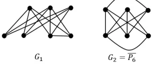
From the above initial conditions, the solitary waves are propagated rightwards. Shapes of both waves at timest= 10,15,20,25and withh=τ = 0.1are shown in Figure 2. We see that as the time progresses the collision occurs and after collision two waves leave each other without changing their shape.
6. Conclusion
Figure 2: The numerical solutions of two solitary waves withh=τ = 0.1obtained at final timest= 10(left-top), t= 15(right-top),t= 20(left-bottom) andt= 30
(right-bottom).
References
[1] S. K. Chung, S. N. Ha, Finite element Galerkin solutions for the Rosenau equation,Appl. Anal.54(1994)39−56.
[2] G. Ebadi, A. Mojaver, H. Triki, A. Yildirim, A. Biswas, Topological solitons and other solutions of the Rosenau-KdV equation with power law nonlinearity, Romanian J. Phys.58(2013)3−14.
[3] A. Esfahani, Solitary wave solutions for generalized Rosenau-KdV equation, Commun. Theor. Phys.55(2011)396−398.
[4] J. Hu, Y. Xu, B. Hu, Conservative linear difference scheme for Rosenau-KdV equation,Adv. Math. Phys.2013, Art. ID 423718, 7 pp.
[5] Y. D. Kim, H. Y. Lee, The convergence of finite element Galerkin solution for the Rosenau equation,Korean J. Comput. Appl. Math. 5(1998)171−180.
[6] P. Rosenau, A quasi-continuous description of a nonlinear transmission line, Phys. Scr.34(1986)827−829.
[7] P. Rosenau, Dynamics of dense discrete systems, Progr. Theoret. Phys. 79
[8] Z. Z. Sun, D. D. Zhao, On the L∞ convergence of a difference scheme for coupled nonlinear Schrödinger equations, Comput. Math. Appl. 59 (2010)
3286−3300.
[9] J. M. Zuo, Solitons and periodic solutions for the KdV and Rosenau-Kawahara equations,Appl. Math. Comput. 215(2009)835−840.
Akbar Mohebbi
Department of Applied Mathematics, Faculty of Mathematical Sciences, University of Kashan,
Kashan, I. R. Iran
E-mail: [email protected]
Zahra Faraz Department of Applied Mathematics, Faculty of Mathematical Sciences,
University of Kashan, Kashan, I. R. Iran
Wiener Polarity Index of Tensor Product of
Graphs
Mojgan Mogharrab
⋆, Reza Sharafdini and Somayeh Musavi
Abstract
Mathematical chemistry is a branch of theoretical chemistry for discus-sion and prediction of the molecular structure using mathematical methods without necessarily referring to quantum mechanics. In theoretical chem-istry, distance-based molecular structure descriptors are used for modeling physical, pharmacologic, biological and other properties of chemical com-pounds. The Wiener Polarity index of a graphG, denoted byWP(G), is the
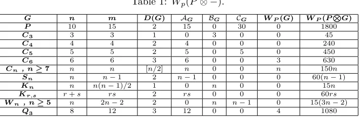
number of unordered pairs of vertices of distance 3. The Wiener polarity index is used to demonstrate quantitative structure-property relationships in a series of acyclic and cycle-containing hydrocarbons. LetG and H be two simple connected graphs, then the tensor product of them is denoted by G⊗H whose vertex set is V(G⊗H) = V(G)×V(H) and edge set isE(G⊗H) ={(a, b) (c, d)|ac∈E(G) , bd∈E(H)}. In this paper, we aim to compute the Wiener polarity index ofG⊗H which was computed wrongly in [J. Ma, Y. Shi and J. Yue, The Wiener polarity index of graph products,Ars Combin. 116 (2014) 235-244].
Keywords: Topological index, Wiener polarity index, tensor product, graph, distance.
2010 Mathematics Subject Classification: 05C20.
1. Introduction
In this section, we first describe some notations which will be kept throughout. A
graph is a structure composed of points (vertices or nodes), connected by lines (edges or links).
A graph is calledfinite if both its vertex set and edge setare finite. If e=uv is an edge of a graph, then we say that e joins the pair vertices uand v. Also
⋆Corresponding author (Email: [email protected]) Academic Editor: Ali Reza Ashrafi
Received 4 July 2016, Accepted 5 September 2016 DOI: 10.22052/mir.2016.34109
c
the vertices u and v are named the end vertices of the edge e. An edge with identical end vertices is calleda loop. We say that a graph issimple whenever it has no loop and no two of its edges join the same pair of vertices. The set of finite simple graphs is shown by Γ and the set of finite graphs in which loops are admitted is denoted as Γ0, so Γ⊂Γ0 [13]. From now on, when we say that
“G is a graph” it means G ∈Γ, otherwise G∈ Γ0. For a given graph G, we
show the vertex and edge set of G by V(G) and E(G), respectively. If x is a vertex of the graph G, the degree of x in G is denoted by degG(x). In the other words, if for any vertex x∈G, NG(x) denotes the set of neighbors that
x ∈ G, i.e. NG(x) = {y∈V (G)|xy ∈ E(G)}, then degG(x) = |NG(x)|. The
minimum and maximum degree of all verticesxof a graphGare denoted byδ(G) and ∆(G), respectively. A walk in G is a sequence of (not necessarily distinct) vertices v1v2 ...vn, such thatvivi+1 ∈E(G)for i= 1,2, . . . , n−1. We call such
a walk a (v1, vn)−walk. A path in the graph is a walk without traversing any
vertex twice. So, a path in the graph is a sequence of adjacent edges without traversing any vertex twice. The graph is calledconnected when there is a path between any pair of vertices in it, otherwise the graph is disconnected. For the verticesu, v ∈V(G), the distance betweenuandv in Gis denoted by dG(u, v)
and it is the length of a shortest (u, v)-path in G. IfGis a disconnected graph, then we assume that the distance between any two vertices belonging to different components of G, is infinity. For a given vertex x ∈ V(G), its eccentricity
ecc(x) is the largest distance between xand any other vertex y ∈ V(G), that is ecc(x) =M ax{dG(x, y)|y ∈V(G)}. The maximum eccentricity over all vertices
of G is called the diameter of G and denoted by D(G). Also, the minimum eccentricity among the vertices of G is called the radius of G and denoted by R(G). LetGand H be two graphs such thatV(H)⊆V(G)andE(H)⊆E(G). Then we say thatH is a subgraph ofGand writeH ≤G. Let us denote a cycle and a path onnvertices byCn andPn, respectively. For a graphH, a graphGis
calledH-free if it has no subgraph isomorphic to H. So, a graph is called triangle free if it has no subgraph isomorphic to C3. Theadjacency matrix of a graph
G, denoted byA(G), is a(0,1)−matrix whose rows and columns are indexed by V(G)and the elementA(G)u,v= 1if and only ifuv∈E(G)for eachu, v∈V(G), otherwiseA(G)u,v= 0.
Mathematical Chemistry is a branch of theoretical chemistry for studying
There exist several types of such indices, especially those based on vertex and edge distances. The most well-known and successful topological indices with several applications in QSAR/QSPR studies in chemistry, was introduced by H. Wiener [27] for acyclic molecules. It is defined as the sum of distances between all pairs of vertices of the molecular graph. LetGbe a simple connected graph. Then theWiener index of Gis defined asW(G) = 12∑x,y∈V(G)d(x, y). Letγ(G, k) be the number of unordered vertex pairs of Gfor which the distance of them is equal tokand therefore one can writeW(G) =∑k≥1kγ(G, k). In the casek= 3, the numberγ(G,3)is called the Wiener polarity index of Gand denoted by WP(G).
It is believed that the Wiener index was the first reported distance-based topo-logical index. This topotopo-logical index was used for modeling the shape of organic molecules and for calculating several of their physico-chemical properties [11]. For example, Wiener used a linear formula to calculate the boiling points of the paraf-fin (alkanes). More precisely, letAbean alkane with the corresponding (Hydrogen suppressed) molecular graphG. Then the boiling point tB(A) of Ais estimated
as follows
tB(A) =aW(G) +bWP(G) +c,
wherea, bandcare constants for a given isomeric group.
Using the Wiener polarity index, Lukovits and Linert demonstrated quanti-tative structure–property relationships in a series of acyclic and cycle-containing hydrocarbons [20]. Hosoya [14] found a physical-chemical interpretation ofWP(G).