This is a repository copy of Solute trapping and the effects of anti-trapping currents on phase-field models of coupled thermo-solutal solidification.
White Rose Research Online URL for this paper: http://eprints.whiterose.ac.uk/83575/
Version: Accepted Version Article:
Mullis, AM, Rosam, J and Jimack, PK (2010) Solute trapping and the effects of anti-trapping currents on phase-field models of coupled thermo-solutal solidification. Journal of Crystal Growth, 312 (11). 1891 - 1897. ISSN 0022-0248
https://doi.org/10.1016/j.jcrysgro.2010.03.009
[email protected] https://eprints.whiterose.ac.uk/ Reuse
Unless indicated otherwise, fulltext items are protected by copyright with all rights reserved. The copyright exception in section 29 of the Copyright, Designs and Patents Act 1988 allows the making of a single copy solely for the purpose of non-commercial research or private study within the limits of fair dealing. The publisher or other rights-holder may allow further reproduction and re-use of this version - refer to the White Rose Research Online record for this item. Where records identify the publisher as the copyright holder, users can verify any specific terms of use on the publisher’s website.
Takedown
If you consider content in White Rose Research Online to be in breach of UK law, please notify us by
Solute Trapping and the Effects of Anti-Trapping Currents on Phase-Field
Models of Coupled Thermo-Solutal Solidification
A.M. Mullis*§, J. Rosam§‡ & P.K. Jimack‡
Institute for Materials Research§ and School of Computing‡, University of Leeds, Leeds LS2 9JT, UK.
Key Words: Solidification: rapid solidification, Phase-field modelling,
Abstract
We explore how the inclusion of an anti-trapping current within a phase-field model of
coupled thermo-solutal growth formulated in the thin interface limit actually affects the
observed levels of solute trapping during dendritic growth. The problem is made
computational tractable by the use of advanced numerical techniques including local mesh
adaptivity, implicit temporal discreteization and a multigrid solver. Contrary to published
results for pure solutal models we find that the inclusion of such an anti-trapping current does
not lead to the recovery of the equilibrium partition coefficient, except in the limit of very
slow growth. At higher growth velocities non-vanishing amounts of solute trapping are
observed.
* Corresponding Author, e-mail : [email protected]
tel : +44-113-343-2568
Introduction
Dendritic growth has been a subject of enduring scientific interest, both because it is a prime
example of spontaneous pattern formation and due to the propensity of many metals to
solidify dendritically from their parent melt. Moreover, remnants of these dendritic
microstructures often survive subsequent processing operations, such as rolling and forging
and thereafter have a pervasive influence on the engineering properties of these metals.
In recent years significant progress towards understanding dendritic growth has been afforded
by phase-field modelling. However, the application of phase-field modelling has largely been
restricted to two limiting cases; namely the thermally controlled growth of pure substances
[e.g. 1, 2]and the solidification of relatively concentrated alloys and solutions [e.g. 3, 4],
wherein growth is sufficiently slow that the problem may be considered isothermal.
However, in the cases of the solidification of very dilute alloys and of rapid solidification
processing the isothermal approximation is no longer valid and it becomes necessary to solve
the problem for coupled heat and solute transport.
Two basic formulations of the coupled phase-field problem have been reported in the
literature. The first, which is due to Loginova et al.[5], follows on from the derivation of the solutal model of Warren & Boettinger[6]. However, there are doubts about the quantitative
validity of this model[7] as the numerical results display excess solute trapping and have an unresolved interface width dependence. This methodology has been extended numerically by
Lan et al.[8], who introduced an adaptive finite volume solver, which allowed them to use realistic values of Le, although this did not overcome either the excess solute trapping or the
interface-width dependence observed in the solution. An alternative formulation of the
coupled phase-field problem based on the Karma thin interface model[9] has been presented by Ramirez & Beckermann[10, 7] and has been extended numerically by ourselves[11, 12] to incorporate a fully adaptive, fully implicit, multigrid solver, allowing higher Lewis numbers
and lower undercoolings to be studied. As the thin interface model has been shown to be
independent of the length scale chosen for the mesoscopic diffuse interface width, it is
radius, ρ. Moreover, the inclusion of an anti-trapping current[9] within this formulation of the coupled problem should ensure that the problems associated with excess solute trapping
observed in the models of [5, 8] are overcome.
For the growth of a dendrite under solute only control it was shown in [9] that the inclusion of
an anti-trapping current effectively totally suppresses solute trapping. However, the growth
velocities observed for solutal dendrites may be very low compared to that for dendrites
growing under coupled thermo-solutal control, and consequently it is not clear what effect the
inclusion of an anti-trapping current within a coupled thermo-solutal model of dendritic
growth will have. That is the subject of this paper.
During equilibrium solidification solute will partition between the solid and the liquid such that the concentrations, and , at the interface location in the solid and liquid phases
respectively are in a fixed ratio, 0
s
c cl0
0 0
l s E
c c
k = (1)
where kE is the equilibrium partition coefficient and can be obtained from the location of the
liquidus and solidus lines on the phase diagram. This partitioning of solute ensures that the
chemical potentials on either side of the interface remain equal. However, as we depart from
equilibrium by increasing the growth velocity, V, either by undercooling the melt or by imposing large thermal gradients to effect rapid heat extraction, the actual ratio
moves away from kE and begins to approach 1. This process of solute trapping has been
shown by Aziz[13, 14] to give rise to a velocity-dependant partition coefficient, k(V), which follows the relationship
0 0
/ l s c
c
β β +
+ =
1 ) (V kE
where β is a dimesionless growth velocity which is generally written as either β = V/VD,
where VD is a characteristic diffusive velocity for atoms at the solid-liquid interface, or as β = Vλ/Di, where λi is a measure of the solid-liquid interface width and Di is an interface
diffusion coefficient. In this latter case β takes the form of an interface Peclet number.
Description of the Model
The starting point for our investigation into the extent of solute trapping within coupled
thermo-solutal phase-field models of solidification is the definition of a free energy
functional,
dV c
T c f
V
c
2 2
) , ,
(φ +σ ∇ 2 +σφ ∇φ2
=
∫
F (3)
where φ(x, t) is the phase variable, which takes values +1 in the solid phase and -1 in the
liquid phase, c(x, t) is the local concentration of component B in A and T is the absolute
temperature. σc and σφ are the gradient entropy coefficients which ensure the increase in
entropy throughout solidification, although here, as in most other phase-field simulations, we
assume σc = 0, while σφ is related to the width of the diffuse interface, W, via the relation σφ = W2H. f(φ, c, T) is the local free energy which may be written,
) , , ( )
, ( ~ ) , ,
( c T f T f c T
f φ = φ M + AB φ (4)
where the first term on the right-hand side is the sum of the free energies of the pure materials
with melting temperature TM, and has the standard form of a double-well potential with barrier
height H,
⎟ ⎟ ⎠ ⎞ ⎜
⎜ ⎝ ⎛
− =
2 4 )
, (
~φ φ4 φ2
H T
while the second term is the free energy due to the solute addition. The form of fAB(φ, c, T)
has been derived in [10] and [15] on the basis of the equilibrium properties that follow from
the two conditions
E
c µ
δ δ
=
F
and =0
δφ δF
(6)
where µE is the spatially uniform value of the chemical potential. The first condition is used
to determine the form of the equilibrium partition coefficient, kE, and the equilibrium
concentration profile while the second leads to the form of fAB(φ, c, T), which is given as,
) ) ( ~ (
) ln ( ))
( ~ 1 ( 2 ln exp )
, , (
2 1
0 0
ε φ ε
ν φ
ν
φ ∆ + − + + ∆
⎭ ⎬ ⎫ ⎩
⎨
⎧ +
= k g T RT c c c c g
m RT T c
fAB M E M (7)
where R is the universal gas constant, ν0 is the molar volume (which we assume constant), m
is the slope of the liquidus line, ∆T = TM - T is the undercooling. g~(φ) is an interpolating
function that satisfies the conditions g~(±1)=±1 and g~′(±1)=0 , and
2 ~ ~
l s ε ε
ε = + , ∆ε =ε~s −ε~l (8)
where ε~ and s ε~ are the free energy densities of the pure solid and pure liquid phases l
respectively.
The evolution of the phase and concentration fields are given by
δφ δ φ
φ(T) F
K t =−
∂ ∂
(9)
and
⎟ ⎠ ⎞ ⎜
⎝
⎛ −
∂ ∇ ⋅ ∇ = ∂ ∂
at
c j
c K t
c δF
where Kφ is the atomic mobility at the interface and
) (
0 φ
ν
Dq RT K
M
c = (11)
where D is the diffusivity of the solute in the liquid phase and q(φ) is an interpolating
polynomial that describes how the diffusivity varies across the solid-liquid interface. For an
asymmetric system, which is appropriate to solute transport (i.e. the diffusivity in the solid is
very much smaller than that in the liquid), we require q(1) = 1 and q(-1) = 0.
Here the first term inside the bracket in Eq. (10) is a manifestation of Fick's law for diffusion
in the liquid while the second term is an anti-trapping current as first proposed by [9], which
takes the form,
φ φ φ
∇ ∇ ∂ ∂ −
−
= ∞
t We k ac
jat (1 E) u (12)
where c∞ is the far-field solute concentration, a is an adjustable parameter which controls the magnitude of the anti-trapping current, the value of which will be discussed later and u is a
dimensionless variable given by
] 1 ) ( [ ln ln
] 1 ) ( ~ [ ln ln
2 1 2
1 − +
⎟⎟ ⎠ ⎞ ⎜⎜ ⎝ ⎛ → + −
⎟⎟ ⎠ ⎞ ⎜⎜ ⎝ ⎛ =
∞ ∞
φ
φ k h
c c g
k c
c
u E E (13)
Here the interpolating function g~(φ) may be replaced by the function h(φ). This is permitted
as ~g(φ) enters into the equations for the evolution of both the phase and concentration fields,
but the actual requirements on the interpolating function are less stringent in the concentration
equation than in the phase equation[15]. Specifically, while it is still required that h(±1) = ±1, we do not require h'(±1) = 0, which subsequently allows the simpler choice h(φ) = φ to be
The purpose of the anti-trapping current is to provide a solute flux normal to the diffuse
interface from the solid into the liquid thus counterbalancing the tendency of phase-field
models to display unphysically high levels of solute trapping. This tendency for solute
trapping is an inherent property of diffuse interface models that do not include an
anti-trapping current and gives rise to a level of solute anti-trapping that is dependant upon the width
chosen for the diffuse interface. As the interface width is generally set considerably larger
than could be considered physical, excess amounts of solute trapping result.
Evaluating the variational derivative (8) and applying the non-dimensionalisations
E u k e U − − = 1 1 and p c L mc T / ∞ − ∆ =
θ (14)
where m is the slope of the liquidus line, L is the latent heat on fusion and cp is the specific
heat, the phase and concentration equations may be obtained as[10]
) )( ( ) ( 2 2 U Mc g f W
t = ∇ − ′ − ′ + ∞
∂
∂φ φ φ λ φ θ
τ (15)
and
{
( )[1 (1 ) ]}
2 1 ] ) 1 ( 1 [ ) ( 2 1 U k h t t U k aW U Dq t U k E E
E + −
∂ ∂ + ⎟⎟ ⎠ ⎞ ⎜⎜ ⎝ ⎛ ∇ ∇ ∂ ∂ − + + ∇ ⋅ ∇ = ∂ ∂ + φ φ φ φ
φ (16)
where M is the scaled slope of the liquidus line,
p E c L k m M / ) 1 ( − −
= (17)
m Hc
L k RT
p E M
0 2
) 1 ( 8
15
ν
λ =− − (18)
τ is a characteristic time for attachment at the interface,
H T
K ( )
1 φ
τ = (19)
and g(φ)=8~g(φ)/15.
Finally, the temperature equation is just the standard thermal diffusion equation with a source
term, namely
t
t ∂
∂ + ∇ = ∂
∂θ α θ φ
2 1 2
(20)
In order to formulate the phase-field model in such a way that the results do not depend upon
the width, W, of the diffuse interface the thin-interface analysis is applied, in which the
system is transformed onto a local orthogonal curvilinear co-ordinate system (ξ1, ξ2, ξ3) which
co-moves with the interface and in which ξ3 measures signed distance from the level line
φ = 0. Asymptotic expansions of the solution,
K + +
+
= 2 2
1
0 φ φ
φ
φ p p
K + +
+
= 2 2
1
0 pU p U
U
U (21)
K + +
+
= 2 2
1
0 θ θ
θ
θ p p
on the inner and outer regions of the solid-liquid interface are matched to obtain an equation
set in which the solution is independent of the width of the diffuse interface. Here, p is a
⎟ ⎠ ⎞ ⎜ ⎝ ⎛ − =
2 tanh 0
η
φ (22)
where η = ξ3/p and we use the convention
0 !
1
=
∂ ∂ =
p k k
k
p k
θ
θ (23)
which is also applied to both U and φ.
Physically, this analysis corrects for the effects of lateral concentration gradients along the
interface, interface stretching (the fact that when curved a diffuse interface is longer on one
side than the other) and the excess solute trapping described above.
The analysis has previously been presented for a coupled model by [10], wherein results
identical to that for the solute only case studied in [9] were recovered. For this reason we do
not here repeat the analysis, only drawing attention to some points that we consider salient to
a discussion of solute-trapping phenomena within the coupled phase-field model.
Specifically, we note that the first order (in p) solutions for U and θ are,
[
+ −]
∫
(
′)
′+
= η φ η η
0 0
0 2
1 1
1 U 1 (1 k )U p ( ) d
U E (24)
η η φ η
θ
θ = + θ +
∫
η ′ d ′Le
A ( )
2 1
0 0
1
1 (25)
where p(φ0) is the function
) (
1 2
) ( ) (
0 0 0
0
φ φ
φ η
φ
q a h
p
− −
= ∂
∂
and Eq. (24) is the same as that obtained for the thin interface analysis of the isothermal solute
problem[9]. If we now adopt h(φ) = φ, this being the simplest function that satisfies the
restrictions on h above, and a = 1/(2√2) which has been shown in the isothermal case to
eliminate the jump in chemical potentials on either side of the interface[15, 9], with q(φ) =
½(1-φ) as defined above we have p(φ0) = (φ0 - 1). That is, the form of the integral in Eq. (24)
reduces to the same form as that in Eq. (25), which is the also the same form as in the thin
interface analysis of the pure thermal problem.
In the isothermal model other values of a are permitted should non-zero amounts of solute
trapping be desired, a point specifically comment upon by [9], although this does require a
re-evaluation of the integral
(
φ η)
η η ηφ
φ η p d d
g
K ( ) ( )
0 0
0 0
∫
−+∞∞∫
⎥⎦⎤ ⎢⎣
⎡ ′ ′
∂ ∂ ′
= (27)
However, in the coupled model the situation is more restrictive in that we require Ui and θi to
have the same form in order for the analysis to be tractable, a point that is perhaps not clear in
the derivation of the coupled model presented in [10], as the substitution h(φ) = φ and
a = 1/(2√2) have already been made when the integrals for U1 and θ1 are formulated.
However, the implication of this is that once the choice h(φ) = φ has been made, the thin
interface analysis for the coupled thermo-solutal model can only be performed for a = 1/(2√2)
and that this is therefore the only value for which the model is valid. Understanding how the
anti-trapping current with a = 1/(2√2) effects the solute trapping behaviour of the coupled
model is therefore an important issue.
Following the thin-interface analysis given in [10] we arrive at the equations governing the
evolution of the coupled concentration, thermal and anisotropic phase fields,
[
]
(
)
⎟ ⎠ ⎞ ⎜ ⎝ ⎛ ∂ ∂ ′ ∂ ∂ + ⎟⎟ ⎠ ⎞ ⎜⎜ ⎝ ⎛ ∂ ∂ ′ ∂ ∂ − + − − − + ∇ ⋅ ∇ = ∂ ∂ ⎥⎦ ⎤ ⎢⎣ ⎡ + + − ∞ ∞ x A A y y A A x U Mc A t U k Mc Le A E φ ψ ψ φ ψ ψ θ φ λ φ φ φ ψ φ ψ ) ( ) ( ) ( ) ( ) ( ) 1 ( ) 1 ( ) ( ) 1 ( 1 1 ) ( 2 2 2 2 2 (28) ⎟ ⎠ ⎞ ⎜ ⎝ ⎛ ∂ ∂ − + + ⎟⎟ ⎠ ⎞ ⎜⎜ ⎝ ⎛ ∇ ∇ ∂ ∂ − + + ∇ − ⋅ ∇ = ∂ ∂ ⎟ ⎠ ⎞ ⎜ ⎝ ⎛ + − − t U k t U k a U D t U k k E E E E φ φ φ φ φ φ ) 1 ( 1 2 1 ) 1 ( 1 2 1 2 1 2 1 (29) t t ∂ ∂ + ∇ = ∂∂θ α θ φ
2 1 2
(30)
where ψ = arctan(φx/φy) is the angle between the normal to the interface and the x-axis and
A(ψ) = 1 + ε.cos(ηψ) is an anisotropy function with strength ε and mode number η. The
characteristic length and time scales are given by
2 1 0 0 a a D d
W = ,
2 1 3 2 2 0 0 Da a d λ
τ = (31)
The dimensionless coupling parameter, λ, results from the thin interface analysis and is given
as[10, 9],
0 0 1 2 d W a a D = =
λ (32)
where d0 is the chemical capillary length and the constants a1 and a2 are given by
8 2 5
1 = =
J I
a , 0.6267
2 2 = + = J FJ K
a (33)
η η φ
d I
2 0
∫
−+∞∞ ⎥⎦⎤ ⎢ ⎣ ⎡
∂ ∂
= (34)
η η φ
φ ∂
∂ ∂ ′
=
∫
+∞∞
− ( )
0 0 g
J (35)
(
φ)
dηF 1
0 0
∫
+∞ += (36)
Numerical Methods
The governing equations are descritized using a finite difference approximation based upon a
quadrilateral, non-uniform, locally-refined mesh with equal grid spacing in both directions.
This allows the application of standard second order central difference stencils for the
calculation of first and second differentials, while a compact 9-point scheme has been used for
Laplacian terms, in order to reduce the mesh induced[16] anisotropy. The mesh data is stored
in a quadtree data structure as in [17, 18].
In order to ensure that sufficient levels of refinement occur around the interface region and
that the extreme multi-scale nature of the thermal and solutal diffusion fields at high Lewis
numbers are handled appropriately, adaptive refinement is based upon an elementwise
gradient criterion given by
(
φ θ)
ν ∇ + ∇ + ∇
=h EC U ET
E (37)
where h|ν| is the element size on the finest level of refinement and EC and ET are user-defined
constants which control the respective effect of the concentration and thermal fields relative to the phase-field. These are compared to two tolerances, and . If, at any location
within the domain the mesh is refined at that location while conversely if
the mesh is permitted to coarsen at that location (subject to geometric constraints). In order to +
Tol
E ETol−
+
≥ETol
guarantee that the solution is sufficiently resolved, a number, Ns, of extra (safety) layers of
elements may be added to those marked by the gradient criterion at each level.
As discussed elsewhere[19, 20] if explicit temporal descretization schemes are used for this
problem the maximum stable time-step is given by ∆t≤ Ch2, where C = C(λ, Le, ∆T), with
C≤0.001 found under certain conditions leading to unfeasibly small time-steps.
Consequently, an implicit temporal descretization is employed here based on the second order
Backward Difference Formula, which is an implicit linear 2-step method, with variable
time-step. Rewriting Equations (28) - (30) in operator form
(
)
⎟ ⎠ ⎞ ⎜ ⎝ ⎛ ∂ ∂ = ∂ ∂ ⎟ ⎠ ⎞ ⎜ ⎝ ⎛ ∂ ∂ = ∂ ∂ = ∂ ∂ t t F t t U t F t U U t F t U φ θ θ φ φ θ φ φ θφ , , , , , , , , , , (38)
the second order Backward Difference Formula (BDF2) with variable time-stepping can be
written as
(
)
(
)
(
)
⎥⎥ ⎥ ⎦ ⎤ ⎢ ⎢ ⎢ ⎣ ⎡ ∆ = ⎥ ⎥ ⎥ ⎦ ⎤ ⎢ ⎢ ⎢ ⎣ ⎡ + + ⎥ ⎥ ⎥ ⎦ ⎤ ⎢ ⎢ ⎢ ⎣ ⎡ + − ⎥ ⎥ ⎥ ⎦ ⎤ ⎢ ⎢ ⎢ ⎣ ⎡ + + + + + + + + + + + + + − − − + + + 1 1 1 1 1 1 1 1 1 1 1 1 1 1 2 1 1 1 , , , , , , , , 1 ) 1 ( 1 2 1 k k k k k k k U k k k k k k k k k k k k k t F U t F U t F t U r r U r U r r φ θ φ φ θ φ θ φ θ φ θ φ θ φ && (39)
where, r = ∆tk/∆tk-1 and the choice of time-steps is based on a set of local error estimators in φ,
U and θ as described in [12]. The method leads to second order convergence in both time and
space and the method can be shown to be A-stable[21], so is therefore appropriate for stiff
systems of differential equations.
When using implicit time discretisation methods on heavily refined finite difference grids it is
necessary to solve a very large, but sparse, system of non-linear algebraic equations at each
time-step. Multigrid methods are among the fastest available solvers for such systems and in
this work we apply the non-linear generalization known as FAS (full approximation scheme
[22]). The local adaptivity is accommodated via the multilevel algorithm originally proposed
operator. For smoothing the error we use a fully-coupled nonlinear weighted Gauss-Seidel
iteration with
(
)
(
)
(
)
ijk k k k ij r r k ij ij k k k k ij k ij U F r U F ij 1 1 1 * 1 1 1 1 1 * 1 1 , , 1 , , 2 + + + ∂∂ − + + + + + + ⎟⎠ ⎞ ⎜ ⎝ ⎛ ⎟ ⎠ ⎞ ⎜ ⎝ ⎛ + − − − = θ φ φ φ θ φ ω φ φ φ φ φ (40)
(
)
(
)
(
)
ijk k k U U k ij r r k ij ij k k k U k ij k ij U F U U r U F U U ij 1 1 1 * 1 1 1 1 1 * 1 1 , , 1 , , 2 + + + ∂∂ − + + + + + + ⎟⎠ ⎞ ⎜ ⎝ ⎛ ⎟ ⎠ ⎞ ⎜ ⎝ ⎛ + − − − = φ φ φ φ ω & & (41)
(
)
(
)
(
)
ijk k k k ij r r k ij ij k k k k ij k ij F r F ij 1 1 1 * 1 1 1 1 1 * 1 1 , , 1 , , 2 + + + ∂∂ − + + + + + + ⎟⎠ ⎞ ⎜ ⎝ ⎛ ⎟ ⎠ ⎞ ⎜ ⎝ ⎛ + − − − = φ φ θ θ θ φ φ θ ω θ θ θ θ θ & & (42) where
(
1 1 1)
(
1 1 1 1)
1* 1 2 1 , , , , , + + + + + + + + + + + ∆ −
= k k k k k
k k k r r U t tF U
Fφ φ θ φ φ θ φ (43)
(
1 1 1)
(
1 1 1 1)
1* 1 2 1 , , , , , + + + + + + + + + + + ∆ −
= k k k k k
U k k k U U r r U t tF U
F φ φ& φ φ& (44)
(
1 1 1)
(
1 1 1)
1* 1 2 1 , , , , + + + + + + + + + + ∆ −
= k k k k
k k k r r t tF
Fθ θ φ φ& θ θ φ& θ (45)
The number of pre- and post-smoothing operations required for optimal convergence has been
investigated within the context of phase-field simulation in [12, 11]. Based on that work we
have used V-cycle iteration with 2 pre- and 2 post- smoothing operations at each level.
A major property of the multigrid method is h-independent convergence, which means that
the convergence rate does not depend on the element size. This behaviour is vital in respect
of being able to solve the extreme multi-scale problem arising from coupled thermo-solutal
phase-field simulations.
Results
Validation of our numerical scheme against both other coupled phase-field models[10, 7] and, where available, against analytical solutions for pure thermal and pure solutal growth have
implementation of the anti-trapping current within the model has been validated by reducing
the coupled model to the pure solutal case at solutal undercooling Ω by setting 1/Le→ 0,
removing Eq. (30) from the equation set and fixing the system temperature everywhere at
θsys = -Ω with Mc∞ = 1 - (1-kE) Ω [see 19]. By so doing it is possible to explore the behaviour
of the anti-trapping current during the growth of a dendrite under solute only control, wherein
we find, in agreement with [9], that solute trapping is suppressed and that the curvature
corrected partition coefficient
] ) 1 ( 1
[ 0
0 ρ
d k k
c c
l
s = − − (46)
recovers the equilibrium partition coefficient, kE, to a very high degree of precision.
Specifically, for Ω = 0.15 and kE = 0.3 we recover k = 0.3000 ± 0.0001, where this has been
tested for λ between 1 and 5 and for h between 0.78 and 0.19 (corresponding to 11 to 13
levels of refinement respectively on a domain of [-800,800]2).
We now consider the partitioning behaviour of the model when we allow a dendrite to grow
under coupled thermo-solutal control. Fig. 1 shows the measured (curvature corrected)
partition coefficient for a large number of simulations as a function of the dimensionless
velocity. All the simulations in this sequence have kE = 0.3, Mc∞ = 0.05, λ = 5 and γ = 0.02
and were run with a fixed minimum grid spacing of h = 0.78, although the domain size varied
between simulations such that interactions between the domain boundary and the thermal
field were not encountered. The growth velocity of the dendrite was controlled by varying the
undercooling, ∆, in the range 0.1 – 0.8. Lewis numbers in the range 200 - 10000 were
considered and are denoted by the symbols in the figure. It is very clear from the figure that
despite the presence of an anti-trapping current the measured partition coefficient varies
strongly as a function of velocity, with the equilibrium value, kE, only being recovered as the
with all the points corresponding to Lewis numbers in the range 200-10 000 laying, to a very
good approximation, on the same curve.
As described above, in experimental solidification studies the observed velocity dependant
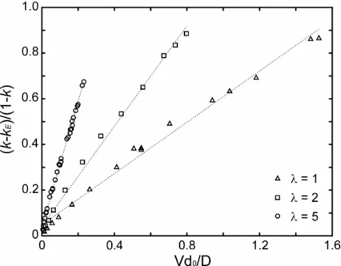
partition coefficient, k(V), is described by the relationship due to Aziz[13, 14] given in Eq. (1). Should this relationship also hold for the phase-field model, plotting the group {(k-kE)/(1-k)}
against V should yield a straight line with gradient 1/VD = λi/Di. A plot of this type is shown
in Fig. 2, where we now also include data for values of the coupling parameters, λ, of 1 and 2
as well as the data shown previously for λ = 5. As before all simulations are run with
kE = 0.3, Mc∞ = 0.05, γ = 0.02 and with a minimum h of 0.78. The Lewis number in the
simulations is, as before, in the range 200 - 10 000, although for clarity we have not indicated
the Lewis number in the plot. This is reasonable as we have already demonstrated above that
there is no explicit Lewis number dependency. A number of points are apparent from the
figure.
Firstly, despite being formulated within the thin interface limit described by [9, 10] the model
does have an interface width dependence in so much as solute-trapping is concerned, with a
more diffuse interface giving rise to higher levels of solute-trapping. Despite this, in respect
of the other main predictive quantities obtained from the model (i.e. V, ρ) the results obtained
from the model are indeed independent of the width of the diffuse interface. This has been
shown both by Ramirez & Beckermann[7] and ourselves[19, 12], with further evidence being presented in Figure 3, where we show that models with different values of λ, and which
therefore display different solute trapping characteristics, give mutually consistent values for
V and ρ. Note that here, due to the requirement to keep the group W0V/D < 1[15], the range of
accessible values of V decreases as λ increases.
The second point that we note is that the data do, to a reasonable approximation, fit the Aziz
model in respect of their velocity dependence. Moreover, if we calculate the slope of the
regression line in each of the three cases we obtain, 0.56, 1.09 and 2.75 (for λ = 1, 2 and 5
of the regression line with λi/Di and noting that λi is the width of the diffuse interface, which
within the phase-field model is W0, itself simply a linear scaling of the coupling parameter λ,
we may obtain Di = 1.81. Similar results can be obtained by varying λ over a wider parameter
space while keeping all other parameters, including ∆, fixed, an example of which is shown in
Fig. 4. Here the model parameters are kE = 0.3, Mc∞ = 0.05, γ = 0.02, ∆ = 0.25, Le = 200 and
we have plotted the group {(k-kE)/V(1-k)} against λ so that, as above, the gradient may again
be directly associated with 1/Di. Here we obtain Di = 1.91 by associate λi with W0 (note
however that 1/gradient of the line is 1.69 as the graph is plotted against λ, not W0, to convert
to W0 the scaling factor of a1 also needs to be applied).
Summary and Conclusions
We have used the phase field model due to Ramirez & Beckermann[7, 10], modified to include an implicit solution capability, to explore how the inclusion of an anti-trapping current within
a model of coupled thermo-solutal growth formulated in the thin interface limit actually
affects the observed levels of solute trapping during dendritic growth. Contrary to published
results for pure solutal models we find that the inclusion of such an anti-trapping current does
not lead to the recovery of the equilibrium partition coefficient, except in the limit of very
slow growth. At higher growth velocities non-vanishing amounts of solute trapping are
observed. Moreover, the extent of this solute trapping is dependant upon the width of the
mesoscopic diffuse interface. Indeed, to a good approximation we find that our model
recovers the Aziz solute trapping law with a constant interface diffusivity, that is that the
solute trapping behaviour may be expressed as a function of the group β = Vλi/Di. This result
has significant implications for the simulation of the growth of dendrites under coupled
thermo-solutal control.
In particular it has hitherto been assumed that provided the phase-field model is constructed
within the thin interface formalism, quantitatively valid results may be obtained independent
of the width of the diffuse interface, leaving this parameter to be chosen for computational
expediency. We now show that this strictly is not the case and that actually λ, and hence W0,
particularly stringent condition as both the results presented here and elsewhere [12, 7, 10]
suggest that V, ρ and σ* do not show a strong dependence on λ, and therefore that they are
only weakly effected by solute trapping. This will be particularly true at low undercoolings,
where the levels of solute trapping are expected to be low. Conversely, at higher
undercoolings and where quantitative predictions of segregation behaviour are required λ may
no longer be considered to be a free parameter, wherein it becomes appropriate to enquire as
to the appropriate value of λ to yield quantitatively valid solute trapping results.
However, obtaining quantitative evidence for what might constitute an appropriate level of
solute trapping is far from straight forward. Experimentally, this is generally presented as a
diffusive velocity (VD = Di/λi), with estimates varying by up to two orders of magnitude in
closely related systems (e.g. from VD = 0.37 m s-1 in Si-As [24] to VD = 32 m s-1 in Si-Bi
[25]). Moreover, there is the possibility that VD is dependant upon kE, with values of kE close
to unity giving values of VD towards the lower end of the spectrum of values. For metal (Al)
based systems, which is probably the closest match to the parameter set used here, [26] have
reported values for VD that may be around 5-20 m s-1. Using the results from above we would
estimate the equivalent (dimensional) diffusive velocity operating here as (1.91/W0)D/d0. We
have shown previously[20] that the parameter set used here is consistent with Cu- 5wt.% Ni, wherein we obtain D≈ 3.2 × 10⁻⁹ m2s-1 [27] and d0 = 3.7 × 10⁻¹⁰ m [28] or VD≈ (19/W0) m s-1.
This would suggest that W0 should be adjusted to be between 1-3 to give realistic values of
solute trapping.
References
1. A.A. Wheeler, B.T. Murray & R.J. Schaefer, Physica D 1993; 66:243.
2. A.M.Mullis & R.F. Cochrane, Acta Mater. 2001; 49:2205.
3. J.A. Warren & W.J. Boettinger, Acta Metall. Mater. 1995; 43:689.
4. J.R. Green, A.M. Mullis & P.K. Jimack, Metall. Meter. Trans. A 2007; 38:1426.
5. I. Loginova, G. Amberg & J. Aagren, Acta Mater. 2001; 49:573.
6. J.A. Warren & W.J. Boettinger, Acta Metall. Mater. 1995; 43:689.
8. C.W. Lan, Y.C. Chang, C.J. Shih, Acta mater. 2003; 51:1857.
9. A. Karma, Phys. Rev. E 2001; 87:115701.
10. J.C. Ramirez, C. Beckermann, A. Karma & H.-J. Diepers, Phys. Rev. E 2004;
69:051607.
11. J. Rosam, P.K. Jimack & A.M. Mullis, J. Comp. Phys. 2007; 225:1271.
12. J. Rosam, P. K. Jimack & A. M. Mullis, Acta Mater. 2008; 56:4559.
13. M.J. Aziz, J. Appl. Phys. 1982; 53:1158.
14. M.J. Aziz, Mater. Sci. Eng. A 1994; 178:167.
15. B. Echebarria, R. Folch, A. Karma & M. Plapp, Phys. Rev. E 2004; 70:061604.
16. A.M. Mullis, Comp. Mater. Sci. 2006; 36:345.
17. N. Provatas, N. Goldenfeld & J. Dantzig, J. Comp. Phys. 1999; 148:265.
18. A. Jones & P.K. Jimack, Int. J. Num. Meth. Fluids 2005; 47:1123.
19. J. Rosam, PhD Thesis, University of Leeds, Leeds LS2-9JT.
20. J. Rosam, P. K. Jimack & A. M. Mullis, Phys. Rev. E. 2009; 79:030601.
21. W. Hundsorfer & J.G. Verwer, Numerical Solution of Time-Dependant
Advection-Diffusion-Reaction Equations, Springer-Verlag, 2003.
22. U. Trottenberg, C. Oosterlee & A. Schuller, Multigrid, Academic Press (2001).
23. A. Brandt,Math. Comp. 1977; 31:333.
24. J.A. Kittl, P.G. Sanders, M.J. Aziz, D.P. Brunco & M.O Thompson, Acta Mater. 2000;
48:4797.
25. M.J. Aziz, J.Y. Tsao, M.O. Thompson, P.S. Peercy & C.W. White, Phys. Rev. Lett.
1986; 56:2489.
26. P.M. Smith, R. Reitano & M.J. Aziz, Mater. Res. Soc. Symp. Proc. 1993; 279:749.
27. X.J. Han, M. Chen & Y.J. Lu, Int. J. Thermophys. 2008; 29:1408.
Fig. 1. Measured partition coefficient, k, as a function of growth velocity for the coupled
thermo-solutal phase-field model with kE = 0.3, Mc∞ = 0.05, λ = 5 and γ = 0.02. Velocity is
varied via altering the undercooling ∆.
Fig. 2. Solute partitioning behaviour as a function of velocity showing good general
agreement with the Aziz model and a dependence upon coupling parameter, λ, (and hence
[image:21.595.71.315.444.635.2]Fig. 3. Dendrite tip radius as a function of velocity for different values of λ, showing that
although λ effects the solute trapping characteristics of the dendrite, mutually consistent
values for the tip velocity and radius are obtained independent of the value used for λ.
Fig. 4. Solute partitioning behaviour as a function of the coupling parameter, λ, showing good
[image:22.595.70.315.464.662.2]