Theoretical Analysis of Stiffness Constant and Effective Mass
for a Round-Folded Beam in MEMS Accelerometer
Wong, W.C. ‒ Azid, I.A. ‒ Majlis, B.Y.
Wai Chi Wong1,2,* ‒ Ishak Abdul Azid1 ‒ Burhanuddin Yeop Majlis3 1School of Mechanical Engineering, Sains University Malaysia
2Department of Mechanical Engineering, College of Engineering, Tenaga Nasional University, Malaysia 3Institute of Microengineering and Nanoelectronic, Kebangsaan University Malaysia
In this paper, the governing equations of stiffness constant and effective mass for a round folded suspension beam in Micro-Electro Mechanical System (MEMS) accelerometer are derived and solved. The stiffness constant is determined by the strain energy and Castigliano’s displacement theorem, whereas the effective mass is determined by the Rayleigh principle. The stiffness constant and the effective mass are solved separately by components and then combined by using the superposition method. The results obtained by the derived equations agree well when compared with the finite element results for several thickness values. The governing equations derived in this paper can be used to predict the natural frequencies and sensitivity of the MEMS-accelerometer.
©2011 Journal of Mechanical Engineering. All rights reserved.
Keywords: effective mass, folded beam, MEMS-accelerometer, stiffness constant, strain energy
0 INTRODUCTION
The development of MEMS devices has become increasingly important since the beginning of the 1990s. MEMS-accelerometers are the most commercially successful MEMS devices [1] and [2]. Among these, the comb finger type capacitive accelerometer is the most successful type of MEMS accelerometer due to its high sensitivity, low drift, stable dc-characteristics, low power dissipation, high bandwidth, simplicity of the fabrication process, absence of exotic materials, and low temperature sensitivity [2] to [5].
Stiffness constant and resonant frequency, which are the topics of this research, are two of the most important functionalities required in the design of any MEMS devices with moving parts. Sensors and actuators in particular, often require a specific stiffness constant and resonant frequency to guarantee successful and repeatable performance. The stiffness constant and effective mass, which incorporate both material properties and physical geometry, characterize the sensitivity and resonant frequency of the MEMS accelerometer. The sensitivity of the accelerometer is a measure of displacement with respect to acceleration. In contrast, resonant frequency characterizes the bandwidth of the accelerometer. The suspension beam can be of
different designs depending on the application of the MEMS accelerometer. However, the study on the structural analysis of suspension beam in the comb finger type accelerometer has not been established well yet. Analytical derivation of these two parameters is only available for simple designs, such as straight beams [5] to [11].
For different geometric shapes, Legtenberg et al. [8] and Zhou and Dowd [9] determined the material properties of the suspension beam and the stiffness constant by using Hooke’s law and the total potential energy, respectively. Tay et al. [10] used the Rayleigh’s energy principle for the determination of resonant frequency as a function of effective mass. Wittwer and Howell [11] used Castigliano’s displacement theorem for the analysis of the vertical deflection due to an applied moment or shear force and the geometric shape. As far as the authors know, the formula for the round folded beam has not yet been derived. Therefore, there is a need to derive the stiffness constant theoretically for a round folded beam to predict the performance of this type of design.
the derivation. From the derived equations, the stiffness constant and effective mass for various parameters are determined and compared with the finite element simulation using ANSYS® 8.1.
1 EQUIVALENT STIFFNESS CONSTANT OF THE SUSPENSION BEAM IN MEMS
ACCELEROMETER
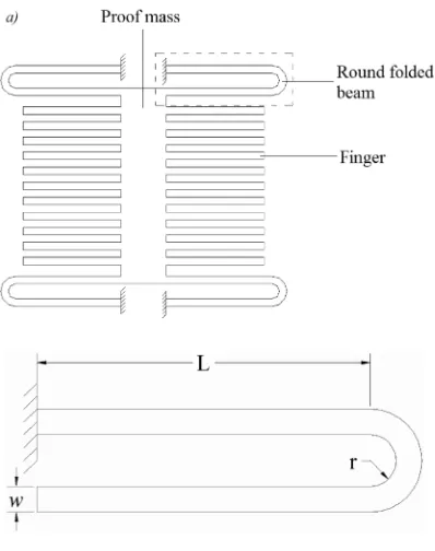
A schematic design of MEMS accelerometer with the round folded beam is shown in Fig. 1a. The close up of the round folded beam with the symbol used in derivation is shown in Fig. 1b, where L is the length of the beam, r is the radius of the round part, and w is the width of the beam.
Fig. 1. Round folded beam as the suspension beam in accelerometer, a) a 2D schematic diagram of MEMS accelerometer, b) the round
folded beam of suspension beam
Fig. 2. Free body diagram of typical arrangement of an accelerometer
In Fig. 1a, the proof mass is suspended by four suspension beams symmetrically at the four edges. The proof mass can be approximated by a central proof mass supported by four springs. The free body diagram of the typical arrangement of an accelerometer can then be approximated by a system of mass and spring as shown in Fig. 2.
In Fig. 2, m is mass of the proof mass; k1,
k2, k3, and k4 are the stiffness constants of each
suspension beam; and x is the displacement. In this spring-mass system, the mass is supported by four springs, thus the external forces are balanced by the four springs evenly and stored as the strain potential energy. The equivalent stiffness constant of the spring-mass system as shown in Fig. 2 can be determined by the following equation of equilibrium:
F mx
k k x k k x mx
x
∑
=−
(
+)
−(
+)
=
,
,
1 2 3 4
(1)
mx k x+ e =0, (2)
where x is the acceleration and Fx is the force.
Therefore, the equivalent stiffness constant, ke = k1 + k2 + k3 + k4.
Since the four suspension beams are in the same dimension and of the same material, then k1 = k2 = k3 = k4 = k1/4 , ke = 4k1/4 , (3)
where k1/4 is the stiffness constant of a quarter
system.
In obtaining the governing Eqs. of the suspension beam for the stiffness constant, the following assumptions are made:
• The proof mass and comb fingers of the structure are rigid.
• The flexible members are attached to perfectly rigid supports.
• The device only vibrates in the sensing axis. • Young’s modulus is constant.
• Damping is ignored.
• 3D effects such as fringing field and comb finger end effects are neglected [12] to [14]. • Euler–Bernoulli beam model assumption is
applied.
2 DETERMINATION OF STIFFNESS CONSTANT IN ROUND FOLDED BEAM
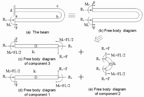
model of the suspension beam together with its boundary condition is shown in Fig. 3a, and its free body diagram is shown in Fig. 3b. In the analysis, the round folded beam can be resolved into three components, with two models of half fixed-fixed beam (Fig. 3c and d) and a model of half ring (Fig. 3e).
Since the device is assumed to vibrate only in the sensing axis, the total displacement of the quarter model δ1/4 is equal to the sum of the
displacement of each component, δ1/4 = δc1 + δc2
+ δc3 .
Based on Hooke’s law (i.e., F = kδ), there is k∝1
δ . In this context, the stiffness constant of the quarter model can be given in a complementary form by:
1 1 1 1
1 4 1 2 3
k =kc +kc +kc , (4)
where kc1, kc2, and kc3 are the stiffness constants
for components 1 to 3, respectively.
2.1 The Stiffness Constant for the First and Third Components
The free body diagram of the first and third components are similar to the model of half fixed-fixed beam subjected to the transverse loading,
as shown in Fig. 4. Fig. 4a shows a fixed-fixed beam with length 2L subjected to a transverse load F at the midspan of the beam. This force causes bending, which could result in reactions at both fixed ends consisting of forces and moments. The maximum displacement δmax occurs at the
midspan of the beam. If this model is cut through its midspan, this part can be modeled as a half fixed-fixed beam. The reactions at both fixed ends are the bending moment M0, shear reaction force
in y-direction Ry, and the axial reaction force in
x-direction Ra, as shown in Fig. 4b. Since the load
is transverse to the axis of the beam, the axial reaction force Ra is extremely small compared to
the bending moment and shear force. Therefore, Ra is ignored in the calculation. The shear reaction
force Ry, and bending moment M0 for the model of
the half fixed-fixed beam is obtained as Ry = F/2
and M0 = FL/4.
The maximum displacement in the model of the half fixed-fixed beam δmax is caused by both
displacement due to bending moment δbm , and the
displacement due to shear δs , or δmax = δbm + δs.
Thus, the stiffness constant of the half fixed-fixed beam is taken as:
1 1 1
khalp kbm ks
= + . (5a)
constant of the half fixed-fixed beam as given in Eq. (5a) as:
1 1 1 1 1
1 3
kc kc khalp kbm ks
= = = + . (5)
2.1.1 The Stiffness Constant Due to Bending
Moment
Fig. 4. Fixed-fixed beam
For a fixed-fixed beam (Fig. 4), the maximum deflection due to a bending moment occurs at the middle of the beam. It is given by [15]:
δbm F L EI
FL EI =
( )
2 =192 24
3 3
. (6)
The stiffness constant due to the bending moment kfull for the full model of the fixed-fixed
beam is then derived as:
k F EI
L
full bm
= =
δ
24
3 . (7)
Thus, the stiffness constant due to the bending moment kbm for the half model of a
fixed-fixed beam is:
1 12
3 k
L EI
bm
= , (8)
where E is the Young’s modulus, I is the second moment of the cross sectional area, and L is the length of the half model of the fixed-fixed beam.
2.1.2 The Stiffness Constant Due to Transverse Force
For a rectangular cross sectional area of width b and depth d, with the total beam length L, and with the applied transverse load of F/2, as shown in Fig. 4b, the maximum deflection (at middle point) due to the shear is given as [15]:
δs F Ls
bdG
= 3
5 , (9)
where G is shear modulus, G= E +
(
)
2 1 µ and μ is the Poisson’s ratio. By knowing Fs = F/2 and by
replacing G and Fs in δs, the maximum deflection
(at middle point) due to the shear is:
δs µ FL
bdE
=6
(
+)
5 1
. (10)
Since ks = F/δs, stiffness constant due to
shear ks in the complementary form is given as
1 6
5 1
k F
L bdE
s s
=δ =
(
+µ)
. (11)2.2 The Stiffness Constant for the Second Component
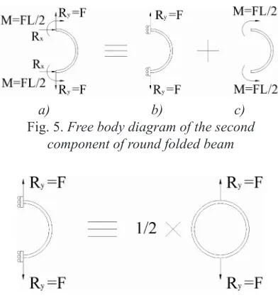
The second component is approximated to be the model of a half ring with simple support on the left, transferred from the first and third components. The free body diagram is shown in Fig. 5a. This component is subjected to two forces, the transverse force Ry and bending moment M.
The stiffness constant of the second component kc2 is the combination of the stiffness constant
due to transverse force kt (Fig. 5b), and stiffness
constant due to bending moment km (Fig. 5c). kt
is approximated to be half of a stiffness constant in the ring kc due to the same value of transverse
force, as shown in Fig. 6.
a) b) c)
Fig. 5. Free body diagram of the second component of round folded beam
2.2.1 The Stiffness Constant Due to Transverse
Force Acting on Half a Ring
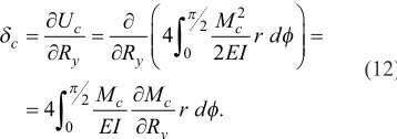
The stiffness constant of the ring component (Fig. 5b) due to transverse force can be determined by using Castigliano’s displacement theorem. The theorem states that deflection at a point on a member in the direction of a force applied at the specific point is given by the partial derivative of the complementary energy with respect to the external force at the point, or
δc = ∂U/∂R, , where U is the internal strain energy
given by U
E dV
V =
∫
12 2
σ . For a beam subjected
to bending, the direct stress is σ = My / I , where M is the bending moment, y is the distance from the neutral axis to the point in question, and I is the second moment of the cross sectional area
I y dA
A =
∫
2 .Thus, U M
EI y dAdx M
EIdx
A
L L
=
∫
∫
22 2 =∫
0
2 0
2 2 ,
where L is the length of the beam. Accordingly,
δc U L
R R
M EIdx =∂
∂ = ∂ ∂
∫
2
0 2 .
For a full ring, the total length is given as
L=
∫
πrdφ=∫
π rdφ0 2
0 2
4 , where r is the radius of
the ring, and ϕ is the angle at any point within the
ring. Since the integration of πdφ
0 2
∫
is always zero, and in view of the symmetry of the ring, only one quadrant of the ring needs to be considered as shown in Fig. 7.Fig. 7. Transverse forces at a ring
According to Castigliano’s displacement theorem, deflection of the ring at any point c is:
δ φ
φ
π
π
c c
y y
c
c c
y
U
R R
M EI r d M
EI M
R r d =∂
∂ =
∂ ∂
=
= ∂
∂
∫
∫
4 2
4
2 0
2
0
2 .
(12)
By cutting the ring at any section within the quadrant of the ring, the bending moment at any point c with an angle of ϕ is given as [15]:
Mc=M0−R r2y
(
1 cos ,− φ)
(13)where M0, the imaginary bending moment, is
unknown but may be obtained from the strain energy.
The strain energy for the quadrant of the ring is:
U
EIM r d
EI M R r
r d
q c
y
= =
= −
(
−)
∫
∫
1 2
1
2 2 1
2 0
2
0
2 0
2
φ
φ φ
π
π
cos .
(14)
The total strain energy for the ring is given by:
U U
EI M R r
r d
c= q= − y
(
−)
∫
4 4 1
2 0 2 1
2
0
2 cosφ φ,
π
(15)
owing to the symmetry at ϕ = 0, ∂U/∂M0 = 0.
Therefore,
1
2 1 0
0 0
2
EI M
R r
r d
y
−
(
−)
=
∫
π cosφ φ . (16)Since 1 / EI ≠ 0 and r ≠ 0,
M0 R r R ry y d
0 2
2 2 0
− +
=
∫
π cosφ φ solved asM0 R ry
2 2 2 1 0
π π
= − −
(
)
. Therefore,M0 R ry 1 2
1
= −
π . (17) Substituting Eq. (17) into Eq. (13), the bending moment at any point c within the full ring, is:
Mc =R ry −
By partial derivative with respect to Ry: ∂ ∂ = − M Ryc r
1 2
1
cosφ .
π (19)
Substituting Eqs. (18) and (19) into Eq. (12),
δ φ
φ
π φ π
π
c c c
y y
M EI
M R r d
EI R r r
= ∂ ∂ = − ⋅ −
∫
4 4 1 2 1 1 2 1 0 2 cos cos = − ∫
∫
rd R r EI d y φ φ π φ π π 0 2 3 2 0 2 4 1 2 1 cos , (20) δ π π π c y R r EI = − + 4 16 1 1 2 3. (21)
Since Ry = F,
δ π
π π
c =4EIFr 16− +1 21 3
. (22)
The stiffness constant of the ring is then given by: 1 4 16 1 1 2 3 k F r EI c = = − + δ π
π π . (23)
Since the stiffness constant for the second component is equal to the half of the stiffness constant of the full ring, kt = ½ kc . Therefore, the
stiffness constant for the second component due to transverse force is given by:
1 2 8
16 1 1 2 3 k k r EI t c = = − +
π π π . (24)
2.2.2 The Stiffness Constant Due to Bending
Moment
The stiffness constant due to the bending moment for this component (Fig. 5c) can be determined by using the energy method. The internal strain energy is:
U
E dV
E
M
I y dA rd E
M I rd M r EI V c A c c = = ⋅ = =
∫
∫
∫
∫
1 2 2 2 1 2 2 2 2 2 0 2 2 2 0 2 2 2 σ φ φ π π ⋅⋅ = π π 2 2 2 2 , .U M r
EIc
E
M
I y dA rd E
M I rd M r EI c A c c = ⋅ = =
∫
∫
∫
2 2 1 2 2 2 2 0 2 2 2 0 2 2 2 φ φ π π ⋅⋅ = π π 2 2 2 2 , .U M r
EIc
(25)
Since the total internal strain energy is equal to the external work performed, U = ½ Fδ ,
then, πM r δ
EIc F
2 2 2
1 2
= .Substituting M = FL/2 into
the equation, FL r
EIc F
2 2 1 2 2 2 π = δ.
By rearranging the above equation, the deflection due to the bending moment is:
δ =πFL r EIc
2 2
4 . (26)
Therefore, the stiffness constant due to the bending moment is given by:
1 4 2 2 2 k F L r EI bm c = δ = π .
Since the width and depth of the second component is equal to the width and depth of the first component,
Ic2 = Ic1 = I, thus 1 4 2 2 k L r EI bm
=π . (27)
2.3 The Effective Stiffness Constant of the Round Folded Beam
The effective stiffness constant of the round folded beam can then be determined from Eq. (3): 1 1 4 1 4 1 1 1 4
1 1 1
1 1
4 1 4
1 2 3
1
k k k
k k k k
k k
e
e c c c
e c = = = + + = + , , kk k
k k k k k k
c c
bm S t bm bm S
2 3 2 1 4 1 4
1 1 1
4
1 1 1
4 1 1 + = = + + + + + = + + + , . 1 1 2 1 2 1 4 1 4 2
ke kbm kS kt kbm
(28)
1 1 2 12 1 2 6 5 1 1 4 8 16 1 3 3 k L EI L bdE r EI e = + ( + ) + + − + µ π π 11 2 1 4 4 24 3 5 1 2 2 3 π π µ + = + ( + ) + L r EI L EI L bdE
r33 2
3 3 3 16 1 1 2 16 1 1 2 3 1 5 24 EI L r EI k Et L w L w r w e π π π π µ − + + = + ( + ) + , rr r L r w 3 2 3 16 1 1 2 3 4 π π π π − + + . (29)
3 DETERMINATION OF EFFECTIVE MASS IN ROUND FOLDED BEAM
The effective mass of the folded beam is determined by using the Rayleigh principle. By taking a beam model with a cross sectional area
A, length L, the displacement at any point x to be
δ(x), and velocity at any point x to be dδ(x)/dt, the maximum displacement δmax is related to the
distribution function N(x) as:
δ(x) = N(x) δmax and d x
dt N x
d dt
δ
( )
δ=
( )
max. (30)The effective mass is given by:
me N x A x dx
L
=ρ
∫
2( ) ( )
0 . (31)
3.1 Effective Mass for Half Model of
Fixed-fixed Beam
Since the distribution function is independent of the applied force, the distribution function can be determined by assuming the half model of the fixed-fixed beam is deflected under a concentrated force F. Displacement at any point within the beam is given by James et al. [16] as:
δ x F
EI Lx x
( )
= −
12 3 2 2 3 . (32)
The maximum displacement occurs at x=L thus,
δmax = FL .
EI 3
12 (33)
Consequently, the distribution function is:
N x x Lx x
L
( )
=δ( )
= −δmax .
3 2 2 3
3 (34)
Effective mass of half model of fixed-fixed beam under bending moment is then given as:
m N x A x dx
A Lx x
L dx A L L x b e L L , =
( ) ( )
= = − = =∫
∫
ρ ρ ρ 2 0 2 3 3 2 0 6 2 3 29 55 6 7
0 6 7 5 12 6 4 7 9
5 2 47 13 35 − + = = − + × = Lx x A L L m L b e ρ ρ ,
, AAL.
(35)
Thus, the effective mass of the first component m1 is equal to that of the third
component m3 or:
m1 m3 mb e 13 AL
35
= = , = ρ . (36)
3.2 Effective Mass for Half Model of Ring For the half model of ring under transverse force (Fig. 5), the displacement at any point within the beam is given by Eq.(20) as:
δ φ
π φ
φ
x R r
EI d y
( )
= − ∫
4 1 2 1 3 20 cos ,
or by expanding:
δ φ φ
π φ
φ π
x R r
EI y
( )
= + − + 4 1 4 2 2 4 1 3 2sin sin . (37)
The maximum displacement is given by
Eq.(21) as δ π
π π
max= − + . 4 16 1 1 2 3 R r EI y
The distribution function:
N x
( )
=( )
x =+ − + − + δ δ φ φ π φ φ π π π π max sin sin 1
4 2 42 1
16 1 21
2
is solved by:
N x
( )
=+
( )
−( )
+ − 1 8 1 16 2 1 1 16 1 2 2 φ φ π φ φ π π π sin sinEffective mass of the half model of the ring under transverse force is then given as:
m N x A x dx
A
a e L ,
sin sin
=
( ) ( )
== +
( )
−( )
+−
∫
ρρ φ φ π φ
φ π π
2 0
2
2
1 8
1
16 2
1
1 16
1 22
2
0 2
π
φ
π
∫
rd .As a result, the effective mass of the second component m2 is:
ρ π π π π
π π π
Ar 6
2 47 32 6144
16 64
7 5 3
2 4 2
+ − −
− +
(
)
. (39)
Thus, the effective mass of the device is
m m m m m n m
m m m n m
e pm f
b e a e pm f
= + + + + =
= + + +
1 2 3
8 , 4 , , (40)
where mpm is the mass of proof mass, mf is the
mass of finger, and n is the number of fingers.
4 COMPARISON RESULTS WITH THE FINITE ELEMENT SIMULATION
The round folded beam in MEMS accelerometer is further analyzed by using the finite element (FE) package, ANSYS® 8.1.
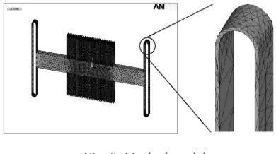
The three-dimensional 20-node structural solid element, SOLID 186, has been used in this analysis. The material properties and the physical geometries used in the FE simulation are shown in Table 1. The FE model meshed by the free meshing is shown in Fig. 8. The simulation result will be used for a comparison with the analytical results obtained by Eqs. (29) and (40).
The resonant frequency is obtained directly from the modal analysis. The stiffness constant is determined by using a static analysis.
Fig. 8. Meshed model
Table 1. Material properties and physical geometries for accelerometer
Elastic modulus kg/µm s127×1032
Poison’s ratio 0.27
Density 2330×10kg/µm3-18 Length of suspension beam (L) 803 mm Width of suspension beam (w) 11 mm
Radius of ring, r 50 mm
Length of comb finger (lfinger) 650 mm
Width of comb finger (wfinger) 15 mm
Number of comb finger 56 pairs Sensing gap distance (d0) 2 mm
Table 2 shows the result of the comparison between the analytical and simulation analysis for stiffness constant and effective mass for several thicknesses (t). From Table 2, it can be seen that the stiffness constant and the effective mass obtained from the derived equations based on the analytical analysis show good agreement with those obtained from the finite element simulation. The difference between analytical and simulation results is below 5%. Based on this, it can be concluded that the derived analytical formulas are capable of obtaining the effective mass and the stiffness constant of the round folded beam of the suspended comb finger type accelerometer. Therefore, they are capable of predicting the resonant frequency and the sensitivity of the accelerometer.
5 CONCLUSIONS
The stiffness constant and the effective mass of round folded beam in MEMS accelerometer have been derived successfully. The derivation of the stiffness constant is obtained by using the strain energy method and the Castigliano’s displacement theorem, while the derivation of the effective mass is determined by using the Rayleigh principle. The result obtained from these derived formulas agree well with the results obtained from FE software ANSYS.
6 ACKNOWLEDGEMENT
provided by the Universiti Sains Malaysia and the Malaysian Government.
7 REFERENCES
[1] Bernstein, J. (2003). An overview of MEMS inertial sensing technology. Sensors Magazine
Online, vol. 20, no. 2, p. 14-21.
[2] Yazdi, N., Ayazi, F., Najafi, K. (1998). Micromachined inertial sensors. Invited Paper, Special Issue of IEEE Proc., vol. 86, no. 8, p. 1640-1659.
[3] Amini, B.V., Ayazi, F.A. (2004). 2.5V 14-bit ΣΔ CMOS SOI capacitive accelerometer. Journal of Solid-State Circuits, vol. 39, no. 12, p. 2467-2476.
[4] Rödjegård, H., Lööf, A. (2005). A differential charge-transfer readout circuit for multiple output capacitive sensors. Sensors and
Actuators A, vol. 119, no. 2, p. 309-315. [5] Borovic, B., Liu, A.Q., Popa, D., Cai, H.,
Lewis, F.L. (2005). Open-loop versus closed-loop control of MEMS devices: choices and issues. Journal of Micromechanics and Microengineering, vol. 15, p. 1917-1924. [6] Chae, J.S., Kulah, H., Najafi, K.
(2002). A hybrid silicon on glass lateral microaccelerometer with CMOS readout circuitry technical digest. IEEE International Conf. MEMS, Las Vegas, p. 623-626.
[7] Lüdtke, O., Biefeld, V., Buhrdorf, A., Binder, J. (2000). Laterally driven accelerometer fabricated in single crystalline silicon.
Sensors and Actuators A, vol. 82, p. 149-154. [8] Legtenberg, R. Groeneveld, A.W.,
Elwenspoek, M. (1996). Comb-drive actuators for large displacements. Journal of
Micromechanics and Microengineering, vol. 6, p. 320-329.
[9] Zhou, G.Y. Dowd, P. (2003). Tilted folded-beam suspension for extending the stable travel range of comb-drive actuators. Journal of Micromechanics and Microengineering, vol. 13, p. 178-183.
[10] Tay, F.E.H., Kumaran, R., Chua, B.L., Logeeswaran, V.J. (2000). Electrostatic spring effect on the dynamic performance of microresonators. Technical Proc. International Conf. Modeling and Simulation of Microsystems, San Diego, p. 454-457. [11] Wittwer, J.W., Howell, L.L. (2004).
Mitigating the effect of local flexibility at the built-in ends of cantilever beams. Journal of
Applied Mechanics , vol. 71, p. 748-751. [12] Tang, W.C, Lim, M.G., Howe, R.T. (1992).
Electrostatic comb drive levitation control method. Journal of Microelectromechanical Systems, vol. 1, p. 170-178.
[13] Li, L. Uttamchandani, D.Ȅ. (2006). Twin-bladed microelectro mechanical systems variable optical attenuator. Optical Review, vol. 13, no. 2, p. 93-100.
[14] Spengen, W.M.V., Oosterkamp, T.H. (2007). A sensitive electronic capacitance measurement system to measure comb drive motion of surface micromachined MEMS devices. Journal of Micromechanics and Microengineering, vol. 17, p. 828-834. [15] Benham, P.P., Drawford, R.J., Armstrong,
C.G. (1996). Mechanics of Engineering Materials. 2nd ed. Prentice Hall Ltd., London.
[16] James, M.L., Smith, G.M., Wolford, J.C., Whaley, P.W. (1989). Vibration of Mechanical and Structural Systems. Happer & Row Publishers, Singapore.
Table 2. Comparison of stiffness constant and effective mass between analytical result and simulation
(ANSYS) result
t [mm] k [mN/mm] meff [×10-7 kg]
Analytical ANSYS % diff Analytical ANSYS % diff
120 59.79 62.01 3.59 4.88 4.72 -3.50
80 39.86 40.46 1.50 3.26 3.13 -4.01
60 29.89 30.39 1.64 2.44 2.35 -3.93