www.ann-geophys.net/30/1371/2012/ doi:10.5194/angeo-30-1371-2012
© Author(s) 2012. CC Attribution 3.0 License.
Annales
Geophysicae
The equatorial ionospheric response over Tirunelveli to the
15 January 2010 annular solar eclipse: observations
C. K. Nayak1, D. Tiwari1,†, K. Emperumal2, and A. Bhattacharyya1
1Indian Institute of Geomagnetism, New Panvel (W), Navi Mumbai-410218, India 2Equatorial Geophysical Research Laboratory (EGRL), Tirunelveli, India
†deceased
Correspondence to: C. K. Nayak ([email protected])
Received: 4 July 2011 – Revised: 9 April 2012 – Accepted: 4 September 2012 – Published: 25 September 2012
Abstract. In this paper we present a case study of the annular solar eclipse effects on the ionization of E and F regions of equatorial ionosphere over Tirunelveli [77.8◦E, 8.7◦N, dip 0.4◦N] by means of digital ionosonde on 15 January 2010. The maximum obscuration of the eclipse at this station was 84 % and it occurred in the afternoon. The E and F1 layers of the ionosphere showed very clear decrease in their elec-tron concentrations, whereas the F2 layer did not show ap-preciable changes. A reduction of 30 % was observed in the
foF1 during the maximum phase of the eclipse. During the
beginning phase of the eclipse, an enhancement of 0.97 MHz was observed in the foF2 as compared to that of the control days. But the foF2 decreased gradually as the eclipse pro-gressed and a decrease of 0.59 MHz was observed towards the end phase of the eclipse. Observed variations in theh0F2 and hmF2 showed lower values than the control days, al-though hmF2 was found to increase a bit during the eclipse. Observed variability in the E, F1 and F2 layer ionospheric parameters on the eclipse day and their departure from the control days are discussed as the combined effect of annular eclipse and presence of counter equatorial electrojet (CEEJ).
Keywords. Ionosphere (Electric fields and currents; Equa-torial ionosphere; Ionospheric irregularities)
1 Introduction
A solar eclipse provides an excellent opportunity to explore the upper and lower ionospheric effects associated with an accurately estimated variation of solar radiation during the eclipse period. Study of the ionospheric response to a solar
eclipse has been in place for decades, and extensive stud-ies have been made with various experimental techniques, such as ionosondes, incoherent scatter radar, rockets, Faraday rotation measurements, global positioning system and satel-lite measurements (Evans, 1965a, b; Klobuchar and Whit-ney, 1965; Rishbeth, 1968; Hunter et al., 1974; Oliver and Bowhill, 1974; Cohen, 1984; Salah et al., 1986; Cheng et al., 1992; Farges et al., 2001; Tomas et al., 2007) as well as the-oretical modeling (Le at al., 2008a, and references therein). Both the measurements and simulations show that the eclipse effect is larger in the midday than in the morning and af-ternoon, and also the decrease in electron concentration is greater in the F1 region than in the E region (Le at al., 2008a). The eclipse effect in the F2 region is larger at high solar activ-ity than at low solar activactiv-ity. In a recent study, the signatures of a total solar eclipse on ionospheric E, F1 and F2 regions, during the forenoon hours, have been reported by Adeniyi et al. (2007), as observed over equatorial station Ilorin, Nige-ria. In the present investigation, we find that the decrease in electron density occurs throughout the E and F1 layer heights at about the same time, while, in the F2 region, the electron density decrease began at lower heights and extended pro-gressively towards the layer peak.
A total solar eclipse during sunset hours on 11 Au-gust 1999 highlighted the eclipse-induced changes in the evening time equatorial E and F regions in terms of sud-den intensification of a weak blanketing Es layer, significant increase inh0F immediately following the eclipse and dis-tinctly different spatial and temporal structures in the spread F irregularities.
Fig. 1. Map describing the detailed path of the 15 January 2010 annular solar eclipse over India and Sri Lanka. The station Tirunelveli is
shown on the map in filled red square.
that the decrease of solar radiation during an eclipse is ex-pected to decrease the electron production rate and hence the electron concentration. However, the F2 layer behavior may be quite different as it is governed by photochemical pro-cesses as well as by electrodynamical and neutral forcing. When the F layer is normally in a state of quasi-equilibrium, the obscured changes in electron density during eclipse are almost entirely due to loss by recombination and production by photoionization (Skinner, 1967).
The annular solar eclipse of 15 January 2010 was partic-ularly interesting in that it occurred near noon, thus avoid-ing the larger portion of normal diurnal variations, and it occurred on a magnetic quiet day of a solar minimum. The path of the annular eclipse that occurred on 15 January 2010 over Tirunelveli is shown in Fig. 1. The observational site Tirunelveli [77.8◦E, 8.7◦N, dip 0.4◦N] has been marked on the map with a red square. The central part of the occurrence of maximum annularity is indicated by the thick black line. The time (in IST) of the occurrence of the eclipse annularity, the sun’s altitude in degrees and its duration are marked on the map. At Tirunelveli, the details of the occurrence time in IST (UT + 5.5 h) on the ground for this eclipse are as follows: the beginning of the eclipse at 11:07:57 IST, maximum mag-nitude of the eclipse at 13:16:51 IST and the end of eclipse at 15:06:52 IST. The maximum obscuration was 84.3 % and eclipse magnitude was 0.918 at this station. The details of the eclipse are available at http://eclipse.gsfc.nasa.gov/SEmono/ ASE2010/ASE2010.html.
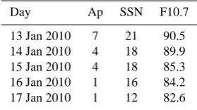
Table 1. Details of parameters during eclipse day and control days.
Day Ap SSN F10.7 13 Jan 2010 7 21 90.5 14 Jan 2010 4 18 89.9 15 Jan 2010 4 18 85.3 16 Jan 2010 1 16 84.2 17 Jan 2010 1 12 82.6
2 Data analysis
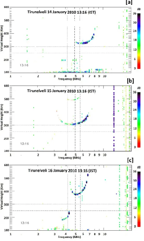
[image:2.595.356.496.384.462.2]Fig. 2. Ionograms recorded at 13:16 IST (when the eclipse
mag-nitude was maximum) on (a) 14 January, (b) 15 January and
(c) 16 January 2010.
[image:3.595.51.288.66.463.2](i.e. foF1,h0F1, foF2,h0F2 and hmF2). For the control days, these parameters were further averaged for 30 min interval. The obtained data show a clear eclipse effect near the begin-ning, maximum and ending phase of the eclipse in the E and F1 regions. This study focuses on the investigation of eclipse-induced changes in the E, F1 and F2 region of the ionosphere. In the E region, the changes in the electron density during eclipse are mainly due to production of electrons by pho-toionization and loss by recombination. However, significant changes in the electron density in the F region may occur due to horizontal and vertical transport of ionization and temper-ature changes along with photochemical reactions. Analysis of photoionization and loss rate will be undertaken and com-municated later.
Fig. 3. Virtual height-time-frequency map observed by CADI at
Tirunelveli on (a) 15 January and (b) 16 January 2010.
3 Results and discussion
For the purpose of comparison, Fig. 2a–c show the iono-grams recorded on 14, 15 and 16 January 2010, at 13:16 IST, the time of maximum eclipse obscuration on the 15th. We can see clearly the absence of E and F1 layer traces and the presence of only F2 trace during the maximum phase of the solar eclipse during the eclipse day. Although the F1 layer critical frequency could be read from the CADI ionograms, the F1 and E layer traces could not be observed by the CADI as the electron density in these layers decreased to below the detection limit due to the solar ionizing radiation being cut down by the eclipse.
The results of the comparisons of the observed eclipse ef-fects on ionospheric E, F1, F2 layers with those of control days are discussed in the following sections.
3.1 E layer
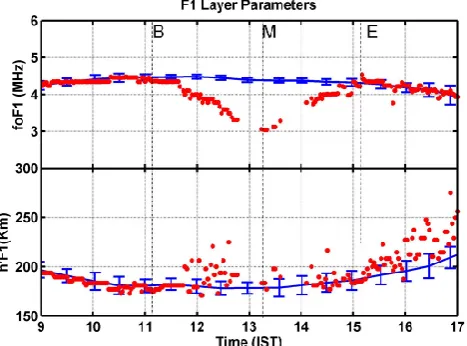
Fig. 4. Top and bottom panels show the temporal variations of the
comparison of foF1 andh0F1 from the control days. The blue line with error bar represents the mean values for the control days. Red stars correspond to the observations of eclipse day.
Normal Es and F1 layer were observed on the control day (i.e. 16 January 2011) during 09:00 to 17:00 IST. Distinctly different features on E and F1 layers of the ionosphere on the eclipse day in comparison with the control day have been noticed. The Es layer has been marked with an arrow. On 15 January 2010, a consistent change begins to be noticed in the Es layer from the onset time (11:07 IST) of eclipse. Es layer became thinner, weaker and disappeared around 11:14 IST and further continued to be weaker till the end of the solar eclipse and continued further till 17:00 IST. Weak blanketing Es was observed 12:44 IST onwards which further intensified around 13:00 IST with maximum fEsb (blanket-ing frequency of Esb layer) around∼7 MHz. This Es ended at 13:04 IST. Sridharan et al. (2002) have also shown the occurrence of blanketing Es during the sunset hours of to-tal solar eclipse on 11 August 1999 and suggested that this could be directly triggered by eclipse phenomena. On iono-grams very weak traces of E layer were present, and hence
foE could not be scaled, indicating the qualitative decrease of foEs and electron concentration.
3.2 F1 layer
Top and bottom panels of Fig. 4 show the comparison of observed temporal variation of foF1 andh0F1, respectively, on the eclipse day with that on the control days. The blue line with error bar represents the mean values of the control days. Red stars represent the eclipse day observations. It is found that the foF1 does not show much day-to-day variabil-ity on the control days, as indicated by their small error bars. The eclipse began around the time period when the range of variation in the foF1 is usually very low, a period of quasi-equilibrium state on normal day. The reduction of solar radi-ation intensity due to the eclipse upset this quasi-equilibrium
electron density) around the maximum phase of eclipse from the control days. In the F1 region, electron densities are con-trolled by the balance between photoionization and chemical recombination. The formation of the F1 layer is mainly due to the altitude variation of the chemical loss (i.e. the tran-sition between αN2 (quadratic) and βN (linear) loss pro-cesses). In the F1 region, the square law lossαN2and linear lossβN are equally important. Lifetime of the electrons in the F1 layer is∼1000 s around 200 km (Banks and Kockarts, 1973). Solar eclipse is a slowly varying process and it took almost four hours to cover the whole eclipse process from eclipse begin to end. The results of Skinner (1967) were for a period of high solar activity when the F1 region is not very distinct from the F2, and 68 % reduction was noticed in the electron density of the F1 region. Adeniyi et al. (2007) have also shown that maximum decrease in the peak elec-tron density as deduced from the critical frequency for F1 was 68 % for the total solar eclipse of 29 March 2006 during low solar activity period. In Fig. 4, the foF1 started decreas-ing around 11:38 IST and a full recovery occurred at about 15:16 IST. The observed duration of decrease of this layer was 3 h 38 min and the eclipse duration was about 3 h 59 min. Observation of consecutive ionograms showed the E and F1 layers fade out during 12:46–13:14 IST and 13:36– 14:06 IST, and resulted as gap in the foF1. The foF1 shows large departure from the normal diurnal variations, ensuring that observed variations were eclipse-induced and are almost entirely due to loss by recombination and production by pho-toionization. With increase of eclipse obscuration, the pro-duction decreases and the loss rate at these heights is in a transition betweenαN2(quadratic) andβN(linear) loss pro-cesses, whereαandβ are the recombination coefficient and N is the electron density (Rishbeth and Garriott, 1969). The observed electron density was minimum around the maxi-mum phase of the eclipse. After this it again increased grad-ually as the eclipse magnitude decreased.
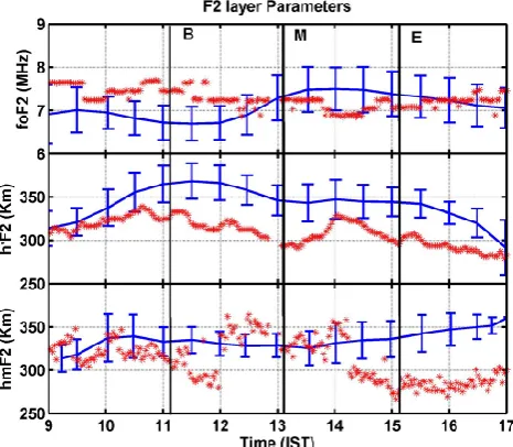
Fig. 5. Top, middle and bottom panels show temporal variations of
the comparison of foF2,h0F2 and hmF2 from the control days. The blue lines with error bar represent the mean values for the control days. Red stars correspond to the observations of eclipse day.
(1967) as a prominent feature of the F region behavior during equatorial eclipses, was not observed during this eclipse.
3.3 F2 layer
The top, middle and bottom panels of Fig. 5 show temporal variation of foF2,h0F2 and hmF2. The blue lines with error bar represent the mean values of the control days. Red stars represent the eclipse day observations. The observed effect of the eclipse on the F2 layer as compared to E and F1 layers is quite different. The maximum observed decrease in foF2 was ∼0.59 MHz around 14:00 IST. In fact, the observed values of the foF2 on the eclipse day are quite similar to those of the control days. From the observations, it is very clear that the values of the foF2 were higher compared to the control days before the onset of the eclipse and the maximum difference was 0.97 MHz. For the control days, it is found that the foF2 increases after 12:00 IST. But, for the eclipse day, no such rise in foF2 is observed. The foF2 starts to decrease around 13:48 IST, and the maximum decrease of∼0.59 MHZ is ob-served just after 14:00 IST. But, if we consider the foF2 be-fore the onset of the eclipse, the actual decrease in foF2 may be higher than the value observed. The differences in foF2 from the control days before the onset of the eclipse were higher, and, following the control days’ trend, it would have been even higher in the absence of the eclipse. However, ob-served values of the foF2 are found to be lower than the con-trol days during the maximum to end phase of the eclipse. The possible reason may be that, during the presence of the eclipse, the ionization production is reduced and the trans-port processes in the F layer are affected due to the presence
of the westward electric field which may in turn lead to the decrease in foF2. The time lag of the maximum decrease of
foF2 with respect to the maximum eclipse obscuration is
ap-proximately 1 h. Also, the observed effect of the eclipse on the F2 layer lasted for approximately 4 h from 12:00 IST to 16:00 IST as shown in Fig. 5. Stations away from the dip equator show the smaller decrease in foF2 (Le et al., 2008a). It should be noted that many previous studies with various measurements (e.g. Datta et al., 1959; Walker et al., 1991; Cheng et al., 1992; Boitman et al., 1999; Huang et al., 1999; Korenkov et al., 2003; Afraimovich et al., 2002; Baran et al., 2003) show that most of the NmF2 (peak electron concentra-tion in the F2 layer) decreases during solar eclipses, whereas the amplitude of foF2 decrease varies greatly from 0.2 MHz to 1.6 MHz. Such a great difference may be induced by back-ground differences in neutral gas and geophysical conditions (such as solar activity and geomagnetic activity level), and by differences in location and local time. In addition, it is pos-sibly due to the measurement methods used with different spatial and temporal resolutions.
Higgs (1942) and Pierce (1948) reported that, during the total solar eclipse of 1 October 1940, there was an increase in foF2 followed by a decrease. Evans (1965b) also found a similar feature of foF2 for the 20 July 1963 total eclipse. Evans proposed two necessary (but possibly not sufficient) conditions for an increase in the foF2 during a solar eclipse: first, the eclipse should be total or very nearly so (>90 %) at F1 region heights; secondly, the magnetic dip should be large (I >60).
Excellent modeling efforts have been made to quantify lo-cal time and solar zenith angle, solar cycle, dip angle, and background hmF2 effects on mid and low latitude ionosphere based on observations made during 7 solar eclipses events from 1970 to 2005 (Le et al., 2008a). Most of the observed differences in behavior of NmF2 during eclipses can be at-tributed to differences in O+loss rate brought about by the background differences in the neutral molecular densities. The F2 region behavior during different eclipse events may be quite different accompanied with various amplitudes of decrease or even a small increase in the electron concentra-tion.
Temporal variation ofh0F2 and hmF2 on eclipse day shows departure from the control days observations. The h0F2 shows a decrease of about∼50 km (15 %) around the eclipse maxima. But an enhancement in hmF2 was observed on the eclipse day. Skinner (1967) and Adeniyi et al. (2007) have shown 50–70 % variation in hmF2 during solar eclipse. From modeling studies, considerable amount of enhancement in the hmF2 is expected on the eclipse day as compared to the control days (Le et al., 2009). But the observed hmF2 does not show much enhancement. The hmF2 increases consider-ably after 12:00 IST and is found to fluctuate till 14:00 IST, and later on it decreased gradually. Although the values of
foF2 were higher than those of control days, still the
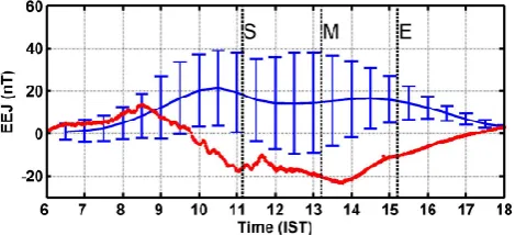
Fig. 6. Temporal variations of electrojet strength for the eclipse and
control days during 06:00–18:00 IST. The blue lines with error bar represent the mean values for the control days averaged for 30 min. Red stars correspond to the observations of eclipse day.
seen in Fig. 6, there is a strong CEEJ from around 10:00 IST to 17:00 IST on the eclipse day. This corresponds to a west-ward electric field which may cause a vertically downwest-ward E×B drift. This does not allow the plasma to be lifted to higher altitudes. It is well established that at equatorial lati-tudes the ionospheric electric fields drive the equatorial elec-trojet and F region plasma drifts that control the development of the equatorial ionization anomaly (EIA), and the genera-tion of ionospheric plasma instabilities (Fejer, 2011, and ref-erences therein).
To understand and explain the observed variability in the h0F2 and hmF2, electrojet strength (1H= Tirunelveli– Alibag of horizontal component of the Earth’s magnetic field), data on the eclipse day (every one minute) along with control days (averaged for every 30 min) are shown in Fig. 6. It is important to note that, on eclipse day, counter equatorial electrojet (CEEJ) was present during 09:47 to 17:00 IST, and maximum CEEJ strength was ∼ −23 nT at 13:45 IST, ob-served shortly after maximum obscuration. Different phase of equatorial electrojet (EEJ) and presence of strong counter-electrojet (CEEJ), its electrodynamics and associated phe-nomena during this solar eclipse have been discussed in de-tail by St. Maurice et al. (2011). They have shown that the electric field turned westward after the time of maximum ob-scurity, reaching its largest westward value one hour before the end of the local eclipse due to the fast eastward-moving local neutral wind dynamo generated by a low pressure sys-tem being triggered by the cold sys-temperatures in the region of maximum obscuration.
Ground-based magnetometer observations of electrojet strength data during daytime have been extensively used to demonstrate the verticalE×B drift velocity in the equato-rial F region in the Peruvian, Filipino and Indian longitude sectors under quiet and disturbed condition during 07:00 and 17:00 IST (Anderson et al., 2006, and references therein). Quiet time1H-inferredE×Bdrift velocities are in excel-lent agreement with the Fejer-Scherliess, quiet time, clima-tological daytimeE×B drift model (Scherliess and Fejer, 1999) in the three longitude sectors.
and it followed the same pattern as that of control days. On the eclipse day, the observed variations in hmF2 do not show large enhancement as expected from modeling studies (Le et al., 2009), although a slight increase in hmF2 was ob-served for the eclipse duration. In a simulation study, Le et al. (2008a) has shown that the equatorward/poleward wind pushes hmF2 upward/downward suggesting that wind direc-tion to be poleward on this particular day. Presence of CEEJ throughout the duration of eclipse shows the presence of the westward electric field in the E region which did not allow plasma to move upward. This explains the behavior ofh0F and hmF2 on the eclipse day.
4 Concluding remarks
This paper presents initial observational results on the equa-torial ionospheric observation during the longest annular so-lar eclipse on 15 January 2010 of this century. Ionosonde data show significant annular solar eclipse effects on E, F1 and F2 layers. Combined effect of annular eclipse and presence of CEEJ are mainly responsible for the variability in the E, F1 and F2 region ionospheric parameters.
Acknowledgements. We thank Observatory and Data Analysis
(ODA) section of Indian Institute of Geomagnetism (IIG), Navi Mumbai for providing electrojet strength data used in this paper. One of the authors (C. K. Nayak) wishes to express his sincere thanks to Indian Institute of Geomagnetism for providing him with a Senior Research Fellowship to carry out this research work.
Editor-in-Chief M. Pinnock and Topical Editor P.-L. Blelly thank two anonymous referees for their help in evaluating this pa-per.
References
Adeniyi, J. O., Radicella, S. M., Adimula, I. A., Willoughby, A. A., Oladipo, O. A., and Olawepo, O.: Signature of the 29 March 2006 eclipse on the ionosphere over an equatorial station, J. Geo-phys. Res., 112, A06314, doi:10.1029/2006JA012197, 2007. Afraimovich, E. L., Kosogorov, E. A., and Lesyuta, O. S.: Effects
of the August 11, 1999 total solar eclipse as deduced from total electron content measurements at the GPS network, J. Atmos. Sol.-Terr. Phys., 64, 1933–1941, 2002.
day-time magnetometer observations, Space Weather, 4, S08003, doi:10.1029/2005SW000193, 2006.
Banks, P. M. and Kockarts, G.: Aeronomy (part-2), Academic Press, 1973.
Baran, L. W., Ephishov, I. I., Shagimuratov, I. I., Ivanov, V. P., and Lagovsky, A. F.: The response of the ionospheric total electron content to the solar eclipse on August 11, 1999, Adv. Space Res., 31, 989–994, 2003.
Boitman, O. N., Kalikhman, A. D., and Tashchilin, A. V.: The mid-latitude ionosphere during the total solar eclipse of March 9, 1997, J. Geophys. Res., 104, 28197–28206, 1999.
Cheng, K., Huang, Y.-N., and Chen, S.-W.: Ionospheric effects of the solar eclipse of September 23, 1987, around the equatorial anomaly crest region, J. Geophys. Res., 97, 103–111, 1992. Cohen, E. A.: The study of the effect of solar eclipses on the
iono-sphere based on satellite beacon observations, Radio Sci., 19, 769–777, 1984.
Datta, S., Bandyopadhyay, P., and Datta, R. N.: Ionospheric obser-vations on the F-region during the solar eclipse of 19 April 1958, J. Atmos. Terr. Phys., 16, 182–185, 1959.
Evans, J. V.: An F region eclipse, J. Geophys. Res., 70, 131–142, 1965a.
Evans, J. V.: On the behavior of foF2 during solar eclipses, J. Geo-phys. Res., 70, 733–738, 1965b.
Farges, T., Jodogne, J. C., Bamford, R., Le Roux, Y., Gauthier, F., Vila, P. M., Altadill, D., Sole, J. G., and Miro, G.: Disturbances of the western European ionosphere during the total solar eclipse of 11 August 1999 measured by a wide ionosonde and radar net-work, J. Atmos. Sol.-Terr. Phys., 63, 915–924, 2001.
Fejer, B. G.: Low Latitude Ionospheric Electrodynamics, Space Sci. Rev., 158, 145–166, 2011.
Higgs, A. J.: Ionospheric measurements made during the total solar eclipse of 1940, October 1, Mon. Not. Roy. Astron. Soc., 102, 24–34, 1942.
Huang, C. R., Liu, C. H., Yeh, K. C., Lin, K. H., Tsai, W. H., Yeh, H. C., and Liu, J. Y.: A study of tomographically reconstructed ionospheric images during a solar eclipse, J. Geophys. Res., 104, 79–94, 1999.
Hunter, A. N., Holman, B. K., Fieldgate, D. G., and Kelleher, R.: Faraday rotation studies in Africa during the solar eclipse of June 30, 1973, Nature, 250, 205–206, 1974.
Klobuchar, J. A. and Whitney, H. E.: Ionospheric electron con-tent measurements during a solar Eclipse, J. Geophys. Res., 70, 1254–1257, 1965.
Korenkov, Y. N., Klimenko, V. V., Bessarab, F. S., Nutsvalyan, N. S., and Stanislawska, I.: Model/Data comparison of the F2-region parameters for the 11 August 1999 solar eclipse, Adv. Space Res., 31, 995–1000, 2003.
Le, H., Liu, L., Yue, X., and Wan, W.: The midlatitude F2 layer during solar eclipses: Observations and modeling, J. Geophys. Res., 113, A08309, doi:10.1029/2007JA013012, 2008a. Le, H., Liu, L., Yue, X., and Wan, W.: The ionospheric responses
to the 11 August 1999 solar eclipse: observations and modeling, Ann. Geophys., 26, 107–116, doi:10.5194/angeo-26-107-2008, 2008b.
Le, H., Liu, L., Yue, X., Wan, W., and Ning, B.: Latitudinal depen-dence of the ionospheric response to solar eclipses, J. Geophys. Res., 114, A07308, doi:10.1029/2009JA014072, 2009.
Oliver, W. L. and Bowhill, S. A.: The F1 region during a solar eclipse, Radio Sci., 9, 185–195, 1974.
Pierce, J. A.: The ionospheric eclipse of October 1, 1940, Proc. IRE., 36, 137–144, 1948.
Rishbeth, H.: Solar eclipses and ionospheric theory, Space Sci. Rev., 8, 543–554, 1968.
Rishbeth, H. and Garriott, O. K.: Introduction to ionospheric physics, Academic Press, 1969, International geophysics series, v. 14, 1969.
Salah, J. E., Oliver, W. L., Foster, J. C., and Holt, J. M.: Observa-tions of the May 30, 1984, Annular Solar Eclipse at Millstone Hill, J. Geophys. Res., 91, 1651–1660, 1986.
Scherliess, L. and Fejer, B. G.: Radar and satellite global equatorial F-region vertical drift model, J. Geophys. Res., 104, 6829–6842, doi:10.1029/1999JA900025, 1999.
Skinner, N. J.: Eclipse effects in the equatorial F-region, J. Atmos. Terr. Phys., 29, 287–295, 1967.‘
Sridharan, R., Devasia, C. V., Jyoti, N., Tiwari, Diwakar, Viswanathan, K. S., and Subbarao, K. S. V.: Effects of so-lar eclipse on the electrodynamical processes of the equato-rial ionosphere: a case study during 11 August 1999 dusk time total solar eclipse over India, Ann. Geophys., 20, 1977–1985, doi:10.5194/angeo-20-1977-2002, 2002.
St.-Maurice, J. P., Ambili, K. M., and Choudhary, R. K.: Lo-cal electrodynamics of a solar eclipse at the magnetic equa-tor in the early afternoon hours, Geophys. Res. Lett., 38, doi:10.1029/2010GL046085, 2011.
Tomas, A. T., L¨uhr, H., F¨orster, M., Rentz, S., and Rother, M.: Observations of the low-latitude solar eclipse on 8 April 2005 by CHAMP, J. Geophys. Res., 112, A06303, doi:10.1029/2006JA012168, 2007.