Method for Integrating Tabular Functions that Considers Errors

(1)

2014; 3(2): 63-67

Published online May 20, 2014 (http://www.sciencepublishinggroup.com/j/acm) doi: 10.11648/j.acm.20140302.14

Method for integrating tabular functions that considers

errors

Vladimir V. Ternovski, Mikhail M. Khapaev

LomonosovStateUniversity, Numerical Math and Cyber Departament, Moscow, Russia

Email address:

[email protected] (V. Ternovski)

To cite this article:

Vladimir V. Ternovski, Mikhail M. Khapaev. Method for Integrating Tabular Functions that Considers Errors. Applied and Computational Mathematics. Vol. 3, No. 2, 2014, pp. 63-67. doi: 10.11648/j.acm.20140302.14

Abstract:

If experimental tables are numerically integrated using quadrature formulas, then the measurement errors of the physical instrument is not taken into account. The result of such numerical integration will be inaccurate because of the accumulation of errors due to the summation of random values, and the residual term of the quadrature formula cannot be calculated using solely classical concepts. The traditional approach consists of applying various smoothing algorithms. In this case, methods are used that are unrelated to the problem of integrating itself, which leads to excessive smoothing of the result. The authors propose a method for numerical integration of inaccurate numerical functions that minimizes the residual term of the quadrature formula for the set of unknown values based on the error confidence intervals by using ill-posed problem algorithms. The high level of effectiveness of this new method, for which it is sufficient to know the error level of the signal, is demonstrated through examples.

Keywords:

Quadrature Formula, Ill-Posed Problem, Tikhonov Regularization

1. Introduction

The data from an experiment make up a set of imprecise values Ω_N ={y₁,y₂,..,y_N} the points of the

}. ,.., , { ₁ ₂ _N

N = x x x

Ψ Set Ω_N may be interpreted as a discrete function of the valuesΨN . Since the errors in

devices are known, there is interest in solving three problems:

(a) Recovering discrete data or a smooth functional dependence.

(b) Numerical differentiation.

(c) Numerical integrating and evaluation of an indefinite integral.

Problems a) and b) are sufficiently covered by A. Tikhonov and his coauthors [1,2] within the theory of ill-posed problems, which cannot be said about problem c). It was noted that the problem of integrating may be well-posed established with appropriate selection of spaces [1]. In this case, the integrated function must be a continuous function. However, the result of numerical integration of a noisy table tells us about the unpredictability, since it is impossible to calculate the error. T.Prvan [3] was the first to pose the question of whether integration is a well-posed problem, and examined the problem of integrating

numerical functions by constructing splines while taking errors into account.

In classical analysis, integration is a well-posed problem. In the theory of functions, Lebesgue integration may be logically interpreted as being the inverse to the differentiation operator. The set of absolutely continuous functions in a given interval coincides with the set of functions represented in the form of an indefinite Lebesgue integral with a variable upper bound of some integrable function plus a constant. However, the indicated property of being the inverse to differentiation is not longer valid a discrete set, since the operation of numerical differentiation is ill-posed.

(2)

,

0 '

∫

= −

a a

dx f dx

f ϕ ϕ

where ϕ(x)∈C₀∞ −is the set of infinitely differentiable functions with compact support, denoted by supp f. Then

,

0 '

const dx f a

=

∫

ϕ

which signifies the ill-posed problem of determining the function f from a first kind equation, if the values of the generalized derivative f' are well-known. Similarly, it is possible to calculate the generalized derivative f' from the equation a

_∫

_f _dx₌_const

0

'_ϕ Note that such ill-posed problems

arise when determining periodic functions according to approximated Fourier coefficients, in which case the Fourier series diverges [4]. Thus, the problem of integrating (differentiating) generalized functions is ill-posed.

Furthermore, the problem of integrating a numerical function with errors cannot be accurately solved using quadrature formulas without considering measurement errors. The proof of this statement may be found in the framework of the classical understanding of integration. The integral of a numerical function with errors does not exist, since there is no limit to which the integral sums converge, insofar as it is impossible to “crush” the partitions. The classical quadrature formula gives an indeterminate result because it is impossible to determine the value of the residual term (which includes second and higher order derivatives) due to the inaccuracy inherent to numerical differentiation of imprecise data.

Note 1. A priori information about the smoothness of suspected dependence is insufficient to calculate the integral. It is necessary to also consider measurement errors and formulate a variational problem to minimize the residual term of the quadrature formula.

Note 2. The fact that integration is an ill-posed problem is understood in the sense of A.N. Tikhonov's definition [1], when the solution is defined ambiguously. In other words, the result depends on the method selected.

The problem of integrating noisy tables (signals) is relevant to an enormous number of applications. Considering measurement errors when integrating tables is the essence of this work. The problem of numerical integration is reduced to a variational one using regularization algorithms [1,2] that take a priori information into account.

2. Noisy Integration

Let the values of an experimental data

{ }

y

i be tabulated

at points xi

, .. 1 , )

(x i N f

y_i= _i +σ_i = (1)

are given with errors σ_i. For random errors simulation Wolfram Mathematica 9.0 is used. Pseudorandom number generator algorithmically create numbers that have some apparent level of randomness.

It is necessary to approximate the integral of the signal (function) f(x_i) for the values

y

_i taking into consideration the errors σ_i. Without loss of generality, consider the method on a uniform grid. For irregular partitions, the following observations will remain valid.

An additional difficulty for numerically integrating tabular data lies in the fact that the values f(x_i) may not be precisely calculated, since the signal dependent error in (1) is only a hypothesis.

Note. The model of random deviations in the relative noise is also considered

, .. 1 ), 1 )(

(x i N f

y_i = _i +σ_i =

in the literature. With this assumption, the zeroes of an unknown function f may coincide with the values of an actual experiment exactly, but still be incorrect.

The application of the standard quadrature formula assumes the existence of a continuous second order derivative or higher of the required dependency f(x)

, ) ( )

(

1

∫

∑

=

+ ≈

b

a

N

k

N k kf x r

a dt t

f (2)

where a_k is the weight, and r_N is the calculation error, which may be only a rough approximation of the integral, since the values of the integrable function

{

f(x_i)

}

are not known and a priori information about errors is not used.

In order to correctly use quadrature formula (2), it is necessary to minimize the calculation errors

r

_N in the set unknown

{

f(x_i)

}

taking into consideration errors

{ }

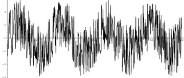
σ_i .

Example. Consider the grid function

k

k k N

y =sin(8

π

(( −1)/( −1)))+

σ

,k=1..N,N =600,

k

σ are pseudo-random integers within the interval

), 2 , 2 (−

i.e., the amplitude of the noise is twice the level of the useful signal (Fig.1a).

Figure 1а. Grid periodic function, “corrupted” with pseudo-random

(3)

Graph of the approximated indefinite integral, calculated using the trapezoidal formula, (Fig. 1b), shows the deviation (drift) -0.181672 of the null value of the integral from the given “function” at the end of interval at k = N.

Figure 1b. Indefinite integral of the function from Figure 1a, calculated using the trapezoidal formula. At k = 600, a summation error appears, which leads to an incorrect value of the integral.

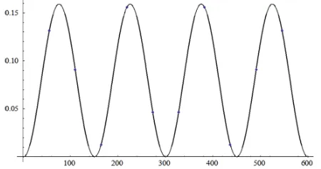
In the following graph (Fig. 1c), the indefinite integral is shown as computed using the trapezoidal formula without accounting for noise.

Figure 1c. Indefinite integral of the original non-noisy function, calculated using the trapezoidal formula.

Thus, ignoring the influence of noise on the quadrature formula leads to an accumulation of errors (displacement of the result) in numerical integration with high probability, even though the oscillations of the signal are smoothed due to the stability of the quadrature formula.

We will discuss the traditional approach to calculating the integrals of functions that are known with errors. At first glance, the integral is calculated using splines [3] for integrand or orthogonal polynomials, and then it is integrated analytically. In this case, the process of analytical integration includes an additional “hyper-smoothing” of the oscillatory interpolant f(x), which can be demonstrated through a simple example.

Let f(x) be replaced with f(x)+εsin(ωx). Then the integration undergoes a smoothing effect

)), cos( ) (cos( )

( )) sin( ) (

(f x x dx f xdx a b

b

a b

a

ω ω

ωε ω

ε = + −

+

_∫

∫

that is, the second oscillating term may be neglected for small amplitudes

ε

or high noise frequencies

ω

.

The fairly trivial inequality (a priori estimate) for the

error of the quadrature formula (2) consists of “theoretical” and “practical” parts.

{ }

∑

=

+ ≤

N

k k i i N

N R a

r

1

max σ , (3)

where the best possible theoretical estimate, or the residual term of the trapezoidal quadrature formula R_N may be presented in a format that is suitable for further study:

∫

=

b

a

N f x dx

h

R ( ) .

8 '' 2

(4)

From inequality (3) it follows that the only possible way to increase the accuracy of numerical integration is to minimize the functional of the residual term R_N (4) in the set of unknown variables f(x_i). In this case, the calculation of the derivative f ''(x) may be performed taking into consideration the known error σ_i using regularization tikhonov methods [1].

Note. Since a const

N

k k ≤

∑

=1

, the quadrature formula (2)

is uniformly stable and is usually used to integrate tabular signals. The result of this operation is inaccurate, since the original function f(x) is unknown.

In order to adjust the numerical integration method to ensure that it is the inverse of the differentiate operator and to correctly calculate the residual term of theoretical error

N

R

, it is necessary to expand the set of differentiable functions, and to interpret the approximation of the derivative as a solution to a Volterra integral equation of the first kind. Thus the function (generalized function) may be discontinuous, but differentiable in the sense that it is the solution to a integral equation of the first kind. Consider, for example, a Volterra integral equation that has a continuous right hand side,

∫

− =

x

x dt t f t x

0

, ) ( ) (

the solution to which is the generalized δ(x) Dirac delta function, which signifies the limit of using the finite-difference approximation of derivatives in tabular data to calculate the residual term R_N . The application of classical formulas of differentiation to approximate the residual term (4) renders it useless in the analysis of approximated data.

3. Constrained Optimization Method

(4)

half of the twentieth century is to correctly calculate R_N

The minimum R_N is a well-posed optimization problem for the conditional extreme of the functional

dx x u S b a U x u ⊂

∫

= min ( ) )

( (5)

on the set of unknown functions u(x_i)= f ''(x_i) , a constraint is imposed in the form of a union of inequalities:

        ≤ − = =

∪

N i i i y x u f U 1 )) (

( σ , (6)

i

x

are fixed nodes of a grid that covers the computational area, ) ( ) ( ) ( ) ( )) (

(u x x u d f' a x f a

f _i x a i i i + + −

=

∫

ξ ξ ξ (7)

i

σ

=max .

The parameter f'(a) may be determined by formula (7) when xN =b through the parameter f(b) . In that case

) (а

f and f(b) stay free (in terms of error) and vary freely (6). When approximating the functional (5) and integral (7), linear and piecewise linear interpolation are used.

Note 1. In the process of minimizing the functional (5), the unknown signal undergoes a restoration (correction), since the residual term (4) acts as a regularization term of the ill-poseed problem. The proof that the conditional minimization problem is well-posed coincides with theorem 2, chapter 2 of [1].

Note 2. When the relative noise of the signal corresponds to formula y_i= f(x_i)(1+σ_i),i=1..N, the constraint (6) in problem (5) is changed to the inequality

        ≤ − = =

∪

N i i i

i y f u x

x u f U 1 ) )) ( ( )) ( (

(

σ

.

Using the

y

_k

=

sin(

8 π

((

k

−

1 )

/(

N

−

1 )))

+

σ

_k from example, σ =2and values f found for the second derivative

i

u , it is not difficult to obtain the values of integral (2) by analytics formulas, using relation (7) or trapezoidal quadrature. The value of the integral was -0.00231485, which was 78 times better than using the classical approach without taking errors into consideration.

To test the accuracy of the proposed method, we examined the problem of integrating an error σk∈[−1,1] equal to null value f(x_k)≡0,k=1..1000 . While the trapezoidal rule gives the integral's value as 0.0748128 at

k=1000, the new method of minimizing the residual term

leads to a “null” error of -2.48715 *10-7.

There is particular interest in the integration of discontinuous digital signals, since classical methods of smoothing are not applicable to such data. To test the method, the function

sign

(

x

)

was selected, with noise

) 4 , 4 (− ∈ k

σ on the interval [−1,1]. The proposed method gave the integral's value as 0.0505905 at 500 nodes, which is an order of magnitude more accurate than the direct application of the trapezoidal method.

Numerical experiments using the Simpson quadrature formula on various noisy digital functions were also performed. The accuracy of integration was also increased when applying the same Simpson’s formula to the set of corrected values of the function taking into consideration the minimization of the residual term. However, there is not big difference between trapezoidal and Simpson’s formulas in the sense of accuracy for noisy tables.

4. Conclusion

The numerical integration of signals given in tabular form is usually conducted using quadrature formulas, and experimental errors are not taken into consideration. In fact, quadrature formulas yield unpredictable results for various reasons. The first reason lies in the impossibility of establishing a priori smoothness of input data, and the second is that there is no way to evaluate the result of integration. Theoretical approximations of the error of quadrature formulas (3) may not be useful for actual values due to the inability to accurately calculate the residual term. The traditional approach consists of applying various smoothing filters. In this case, algorithms are used that do not depend on the task of integrating itself, which leads to excessive smoothing. The authors propose a new method for solving the problem of numerically integrating inaccurate signals that minimizes the residual term of the quadrature formula (4) for the set of unknown values of the signal by using ill-posed problem algorithms [1].

The idea behind the method lies in correcting a table of physical data (within the bounds of known errors) so that the absolute value of the residual term of the quadrature formula corresponds to the true value of the error of numerical integration. In this case, the repeated application of the quadrature formula to the corrected table will increase the accuracy of integration.

The high level of effectiveness of this new method, for which it is sufficient to know the error level of the signal is demonstrated through examples.

References

[1] A. Tikhonov and V. Arsenin, Solutions of ill-posed problems. Winston, Washington, DC(1977).

(5)

[3] T. Prvan , Integrating noisy data, Appl.Math.Lett.(1995) Vol. 8, No.6: 83-87.