IIII
nternational
nternational
nternational
nternational
JJJJ
ournal of
ournal of
ournal of
ournal of
Agriculture and Biosciences
Agriculture and Biosciences
Agriculture and Biosciences
Agriculture and Biosciences
www.ijagbio.com; [email protected]
Research Article
Numerical Simulation of Pounded Area in Drip Irrigation Using by the New
Model of Coupling of Two-Phase Navier-Stokes and Richards Equations
Yaser Yekani Motlagh
1*, Ali AShraf Sadraddini
2, Amir Hossein Nazemi
3and Hossein Rezaie
41,2,3
Faculty of agriculture, Department of Water Engineering, University of Tabriz, Iran
4
Faculty of agriculture, Department of Water Engineering, University of Urmia, Iran
*Corresponding author: [email protected]
Article History: Received: January 28, 2016 Revised: May 22, 2016 Accepted: June 21, 2016
A B S T R A C T
In drip irrigation, different numerical and analytical models such as Hydrus are used for estimation of wetting pattern. In these models, different parameters are considered as inputs which one of these parameters is pounded area. Amount of this parameter could be obtained by experiment or trial and error methods. Therefore, presenting a model that is able to simulate the pounded area in different time steps and is adaptable to the subsurface flow can increase simulation accuracy and reduce the costs of empirical experiments to determine the pounded area in the numerical models in order to specify wetting pattern. In this paper, a new model for coupling surface (Navier-Stokes, VOF) and subsurface flow equations (Richards) is presented. The method can be used for simulation of the both two phase air-water surface and subsurface flows for determining wetting pattern in the soil in surface drip irrigation. In this model, Richards’ equation is discretized with finite volume method and coupled with two- phase Navier-Stokes equations based on a new coupling algorithm. To demonstrate the accuracy of the model, simulation results of soil pounded area in four soil textures and in different discharges were compared to the filed experimental results based on three statistical indices including Mean Error (ME), Root Mean Square Error (RMSE) and Model Efficiency. The results showed that the proposed model has high accuracy to estimate the pounded area and wetting pattern on the soil without field experiments and provided complete data about the velocity, pressure and interface of superficial two-phase flow.
Key words: Drip Irrigation, Equations Coupling, Navier Stocks Equations, Richards Equation, Wetting Pattern
INTRODUCTION
A glance over the history of water and irrigation in the world reveals that several methods for land irrigation have been innovated in recent years. Insufficiency of water, inappropriate atmospheric condition, hilliness, unfavorable quality of water, and lack of access to work force are some limiting factors in development of such methods. Drip irrigation is one of the new methods that has rapidly been developed in different countries. Moisture distribution and wetting pattern of soil in drip irrigation depend to several parameters such as hydraulic specifications of the soil, emitter discharge, evapotrans-piration and architectural shape of root (Lazarovitch et al., 2009). There are various empirical, analytical, and numerical methods for describing water infiltration phenomenon under a point source that estimate the wetting pattern of the soil from its hydraulic
specifications. Some of the researchers in this regard are(Philip, 1971; Ben-Asher et al., 1978; Levin et al., 1979; Philip, 1978; Ben-Asher, 1986; Lafolie et al., 1989; Angelakis et al., 1993; Al-Qinna and Abu-Awwad, 2001; Thorburn et al., 2003; Elmaloglou and Malamos, 2006; Chen et al., 2006; Lazarovitch et al., 2007; Bhatnagarand and Chauhan, 2008; Keyyan and Peters, 2011; Dabral et al., 2012; Zhigang Liu et al., 2015).
Hydrus is a software package for simulating water, heat, and salt movement in two- and three-dimensional variably saturated porous media, presented by Simunek et al., (1999). In this software, Richards’ equation is solved numerically for movement of water in unsaturated soil. Several researchers have used this tool to examine the ability of this model in prediction of wetting pattern in surface and subsurface drip irrigation such as (Skaggs et al., 2004; Cook et al., 2006; Provenzano, 2007; Kandelous and Simunek, 2010; Bufon et al., 2012;
Cite This Article as: Motlagh YY, AA Sadraddini, AH Nazemi and H Rezaie, 2016. Numerical simulation of pounded
Boštjan et al., 2014). The results of these studies indicate that the numerical model of Hydrus has an acceptable accuracy in simulating wetting pattern in surface and subsurface drip irrigations in soils with different textures. Different parameters are considered as input to predict wetting pattern by numerical and analytical models. One of these parameters is pounded area formed on the soil. In fact, when water by a constant discharge is poured to one area of soil, a wet area is appeared. This area is expanded over the time and after a certain duration, a circle area with constant diameter is created. When, diameter of wet circle reaches to a fixed limit, water flow is stable in the soil and this area is called pounded area. One of the problems of analytical and numerical models, especially Hydrus is to specify the pounded area created on the soil; therefore, this area is usually obtained with iterative method or a high cost experimental test. Therefore, presenting a model with ability to simulate the pounded area in different time steps and adjustable to subsurface flow condition is an important issue. One solution to this problem is coupling of surface and subsurface flow equations.
So far, some researchers have employed coupling equations for simulating surface and subsurface flows in surface irrigation and hydrology studies.Morita et al. (2002) presented a model for coupling two-dimensional surface and there-dimensional subsurface flows in order to simulate the procedure of Saint-Venantand Richards’ equations. Panday and Huyakorn (2004 )offered a three-dimensional model for the relationship between surface and subsurface flows applicable to rivers, lakes, ponds and canals. They utilized a two-dimensional zero inertia model for simulating surface flow and Richards’ three-dimensional equation for simulating subsurface flow. Zerihun et al. (2005a, 2005b) presented a numerical model of coupled surface and subsurface flows equations with an ability to couple it with the model of solute transport in soil for applications in basin and border irrigations. Wöhling et al. (2007a, 2007b) provided a numerical model coupling surface and subsurface flow equations in furrow irrigation in a way that root water uptake as a sink term was added to Richards’ equation for accurate simulation of the soil wetting pattern. Kong et al. (2010) presented a new model coupling surface and subsurface flow equations for simulation of flow in coastal areas, providing surface and subsurface flow simulations from Saint-Venant and Dupuit-Forchheimer equations respectively. Kohne et al. (2011) offered a model coupling surface and subsurface flows, applicable in ecological and agricultural systems, which utilized one-dimensional kinematic wave model for simulating surface flow and Richards’ two-dimensional equation for subsurface flow.
In this paper, numerical model of coupling Navier-Stocks and Richards equations has been proposed to estimate the pounded area and exact estimation of wetting pattern. Noting the fact that the presented models by previous researchers are not able to simulate the surface flow and its relevant pounded area in drip irrigation with the presented model, it is possible to predict more accurately surface and subsurface wetting pattern in different soil textures with diverse emitter discharges needless to field experiments.
MATERIALS AND METHODS
Equations for surface and subsurface flows and the method of coupling equations
Surface flow
Equations for two-phase water-air surface flow are continuity equation (1) and Navier-Stokes equation (2), respectively (Hirt et al, 1990).
(1) (2)
In these relations is the dynamic viscosity, density flow velocity, and P is two-phase surface flow pressure (water-air). As surface flow involves two phase of water and air, in this study, VOF model is employed for the two-phase simulation. In this method, a variable is introduced as the volumetric fraction of air in each cell. The volumetric fraction of air is the ratio of air volume to total cell volume. Value of the volumetric fraction of air to each cell is achieved from the following equation (3).
(3) After determining the value of the volumetric fraction of air in each cell, the values of density and viscosity are achieved from (4) and (5) relations.
(4)
(5) So, there is only one of the following states:
0
=
α The cell is empty of air and full of water.
1
=
α The cell is full of air. 1
< <
0 αq The cell is a combination of air and water. The free surface is where the value of α is between zero and one. Therefore, variables and characteristics of each cell is related to one phase or its combination to other phases.
Subsurface Water Flow in Unsaturated Porous Media
The governing Equation for subsurface flow in unsaturated porous media is Richards’ non-linear equation (Richards, 1931). This equation is resulted from the combination of conservation of mass and Darcy’s Law. Generally, the equation is written in the following form.
= .[K(h). (h+z)] (6)
In which is the volumetric water content [L3L-3] as a function of location, h pressure head [L], t time [T] and K unsaturated hydraulic conductivity of soil as a function of pressure head, The Mualem-Van Genucten hydraulic functions (van Genuchten, 1980; Mualem, 1976), as the most widely used functions, were selected in this study.
) 7 (
( )
(
n)
mr s r
h h
α
θ
θ
θ
θ
+ − + =
1
) 8 (
( )
(
)
2 1 1 1 . − − = mm
e l
e
sS S
K h K
n
m
1
1
,
=
−
r s r e S θ θ θ θ − − = (9)Where θs and are saturated and residual water contents, saturated hydraulic conductivity, and n, α, l are shape parameters. Coupling Surface and Subsurface Flow Equations As it is aforementioned, Navier-Stokes and Richards’ equations are utilized for simulating surface and subsurface flow, respectively. To this end, coupling equations is used in this study. According to the flowchart in Figure 1, first, surface flow equations (Navier-Stokes equations) are solved. Boundary condition for Navier-Stokes equations is satisfied by considering the infiltration rate which obtained using potential gradient on interface of water-soil, resulted from solving Richards’ equation in preceding time step. By solving Navier-Stokes equations as two-phase flow model, the interface between air and water is characterized and the velocity and pressure for air and water are determined. Then, the determined water pressures (h) in the nodes of the water- soil interface are used as boundary condition values for solving Richards’ equation in the present time step. This staggered process is followed until achieving to the final result. In this paper, the open source CFD package, Open Source Field Operation and Manipulation (‘OpenFOAM’), which is based on the work of Weller et al. (1998)was used for the flow simulation. The discretisation of the flow governing equations in the ‘OpenFOAM’ is based on the finite volume method formulated with the collocated variable arrangement, with the pressure and velocity solved by segregated methods. Open FOAM is a C++ code library of classes for writing CFD codes, which includes a well-tested and validated RANS capability, and the VOF model for the two-phase flow modeling. Several numerical convection differencing schemes are available in OpenFOAM, including upwind, central difference, QUICK and flux limiters schemes. In this study, the numerical code is developed. Firstly, Richards’ equations are written in C++ programming with finite volume method. Then, it is coupled with two-phase Navier-Stokes equations and VOF method based on presented algorithm. Model Accuracy Assessment Criteria To analyze the simulated values based on the observed data in this study, four statistical criteria of root mean square error (RMSE), coefficient of determination (R2), model efficiency (EF), and mean error (ME) are utilized. Model efficiency relation is presented by Smith et al. (1996). The maximum value of this parameter is one and the closer the EF value to one, the higher the model efficiency. The relations for calculating root mean square error, coefficient of determination, model efficiency, and mean error are: (10)
(11)
(12)
(13) Where Xi and Yi are the observed and modeled values
respectively is the mean of the observed (measured) data and n is the number of observations.
Characteristics of Simulated Numerical Model
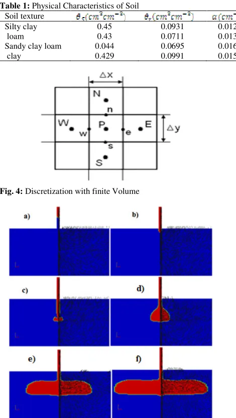
Validity of the numerical model, in this study, is analyzed through field experiment results by Alibabaei et al. (1997). They used four kinds of soils with the shown characteristics in Table 1. Alibabaei et al.(1997) in their field studies measured the pounded area using an emitter with different discharges in different soil textures and periods at 3000 seconds.
Mesh study and Boundary Conditions
In Figure 2, three-dimensional scheme of the simulated flow in this study is presented. This schematic model includes three sectional areas of surface, subsurface flows, and emitter outflow. The solution field is considered a cylinder with 50 centimeters radius and 60 centimeters height in which the height of surface flow section is 2 millimeters (distance of out flowing water from emitter to soil). Dimensions of the emitter are defined as a cylinder with 2 millimeters diameter and 2 centimeters height. As it is clear from Figure 2, the flow domain has a symmetrical geometry to central axis passing from emitter (A-A); therefore, only a sector of the presented domain in Figure 2, is assigned for mesh generation and the problem is solved as a case of axial symmetry. Figure 3, illustrates a section of mesh network near the emitter comprising fields of surface, subsurface and emitter flows. The applied mesh contained structured grids and the number of selected meshes, in this study, is 26500. Moreover, in some part of the mesh network such as near the emitter, for achieving high accuracy the mesh densities are increased.
In this study, according to Figure 3, the location of outflowing water from emitter is considered as the velocity boundary condition at the inlet of system and the velocity is calculated regarding to sectional area of emitter in different discharges. The wall of emitter is considered also as the wall boundary condition and other surface flow boundaries are regarded as boundary condition for atmospheric pressure. Boundary condition of interface flow for surface and subsurface is considered as a boundary condition varying with time and determined from solving the coupled surface and subsurface equations according to the explanations in the previous section. For subsurface flow boundary condition of free drain is considered in lower and side sections.
Numerical solution
Fig. 1: Flowchart for Coupling Surface and Subsurface Flow Equations
Fig. 2: Scheme of Simulated Three-dimensional Model
Fig. 3: Mesh and boundary condition configuration.
(14)
The general equation after time and space discretization is as following: (15)
Where the superscripts n and m denote the time and iteration levels, respectively. A truncated Taylor series for the water content at the new time step and new iteration with respect to h has the form: = + - ) (16)
By substituting of this equation in equation (15), the general form of the resulted linear equation is: + + +p + (17)
= = = = (18)
= - (19)
= - - +( - )( ) (20)
For the right side boundary condition, equation (17) is modified as: P=0, + + + = (21)
=- (22)
= - - + ( - ) ( ) (23)
Also in lower boundary condition, equation (17) can be written as: β=0, + +p + = (24)
RESULTS AND DISCUSSION
Qualitative Results of Surface and Subsurface Flow Simulation (water content volume fraction contours)
Table 1: Physical Characteristics of Soil
Soil texture sand silt Clay
Silty clay 0.45 0.0931 0.0124 0.3901 15.12 0.5 16.6 41 42.4
loam 0.43 0.0711 0.0138 1.413 17.75 0.5 39.4 35 25.4
Sandy clay loam 0.044 0.0695 0.0162 1.3757 41.04 0.5 36.6 26 27.41
clay 0.429 0.0991 0.0157 1.3257 8.84 0.5 14 35 51
Fig. 4: Discretization with finite Volume
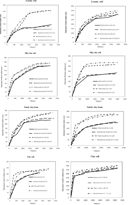
Fig. 5: Qualitative Results of Surface and Subsurface Flow
Simulation with Discharge 2.63 L/h in Soil with loam Texture.
Fig. 6: Qualitative Results of Surface and Subsurface Flow a:
Sandy clay loam soil b: Clay soil
shape of velocity vectors in water and air parts, the air fluid is moving out from the emitter by coming down the water. In figure (5-c), water drop is broken after exiting the emitter and contacting the earth. In figure (5-d), the water flows on the earth without infiltration in the soil after contacting the earth. The velocity vectors in the water section indicate that water flow inside the soil is strongly vortical. According to figure (5-e), in next moments, the water flows on the surface and then infiltrates inside the soil. The level of infiltration flow and
flow discharged into the earth area strongly depends on hydraulic conductivity of soil. As figure (5-f) shows, the pounded area and the water depth inside the soil area will be larger by flowing and infiltrating the water inside the soil. The results show that after a certain time, the radius of pounded area is not changed and just the water infiltrates inside the soil through this area. In fact, this is the same radius which obtained by field experiments and considered as input in the numerical models such as Hydrus. As indicated, the presented model in this study is able to obtain the area directly. In figure (6), the numerical solution results are presented for two kinds of soil including sandy loam and clay textures with different hydraulic features in a certain time and identical discharge (2 L/h). According to the figure, the pounded area of soil with higher hydraulic conductivity (soil with sandy clay loam texture) is smaller than soil with lower hydraulic conductivity (soil with clay texture), but the wetted depth in clay loam soil is more. For more survey, the simulated qualitative results conducted on different textures and discharges of soils are presented in following to confirm the results.
Quantitative results of numerical simulation for wetting pattern advance
The radius of pounded area as a function of time with different discharges and in different textures is compared to the experimental results in figure (7). The results of these figures reveal that the results provided by the model are consistent to the field results. Moreover, these figures show that the radius of pounded area was increased immediately and reached on a fixed value after 10-15 minutes. The radius is increased by decreasing hydraulic conductivity so that heavier soil texture increases the pounded area radius. The figures confirm that the time needed to reach steady state is increased by increasing the discharge of emitter.
Precision Assessment of the presented Model
Table 2: Mean squared error values, efficiency values and coefficient of determination in different soil textures and discharges between field values and values resulted from presented numerical model
R2 EF RMSE q(lit/hr) Soil texture
0.998 0.996 2.80 0.52 loam
0.991 0.976 9.27 1.63 loam
0.967 0.991 9.31 2.62 loam
0.971 0.982 14.30 3.06 loam
0.998 0.998 2.10 0.90 Silty clay
0.997 0.996 3.16 1.03 Silty clay
0.984 0.988 8.67 2.30 Silty clay
0.998 0.999 9.49 4.10 Silty clay
0.967 0.959 8.10 0.58 Sandy clay loam
0.992 0.993 3.86 1.44 Sandy clay loam
0.993 0.996 4.03 3.00 Sandy clay loam
0.978 0.985 10.59 5.31 Sandy clay loam
0.987 0.987 7.85 0.50 Clay
0.968 0.997 12.86 0.80 Clay
0.996 0.998 6.47 1.29 Clay
0.972 0.973 21.35 1.45 Clay
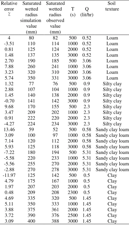
Table 3: Percent of relative error for estimated values with
presented numerical model and field values Relative error ٪ Saturated wetted radius simulation value (mm) Saturated wetted radius observed value (mm) T (s) Q (lit/hr) Soil texture
4 80 82 500 0.52 Loam
-3.51 110 114 1000 0.52 Loam
0.81 125 124 2000 0.52 Loam
1.48 137 135 3000 0.52 Loam
2.70 190 185 500 3.06 Loam
7.88 260 241 1000 3.06 Loam
3.23 320 310 2000 3.06 Loam
5.74 350 331 3000 3.06 Loam
1.32 77 76 500 0.9 Silty clay
2.88 107 104 1000 0.9 Silty clay
1.45 140 138 2000 0.9 Silty clay
-0.70 141 142 3000 0.9 Silty clay
9.68 170 155 500 2.3 Silty clay
3.47 209 202 1000 2.3 Silty clay
0.91 222 220 2000 2.3 Silty clay
-4.27 224 234 3000 2.3 Silty clay
13.46 59 52 500 0.58 Sandy clay loam
3.09 100 97 1000 0.58 Sandy clay loam
7.14 120 112 2000 0.58 Sandy clay loam
5.93 125 118 3000 0.58 Sandy clay loam
-7.22 180 194 500 5.31 Sandy clay loam
-5.58 220 233 1000 5.31 Sandy clay loam
-5.56 255 270 2000 5.31 Sandy clay loam
-2.88 270 278 3000 5.31 Sandy clay loam
-11.97 125 142 500 0.5 Clay
4.79 175 167 1000 0.5 Clay
1.97 207 203 2000 0.5 Clay
0.48 209 208 2300 0.5 Clay
4.69 335 320 500 1.45 Clay
5.11 350 333 1000 1.45 Clay
3.88 375 361 2000 1.45 Clay
3.72 390 376 2500 1.45 Clay
3.09 400 388 3000 1.45 Clay
Conclusion
In this study, a new model to estimate the soil wetting pattern in surface drip irrigation is presented with coupling the Navier-Stocks and Richards’ equations. In simulation of the soil moisture pattern under a water
source, most of the relevant models need estimation of the surface ponded area for using as the upper boundary condition, which is usually determined through a trial and error method or field experiments. This study attempts to develop a model which does not require to estimation of the mentioned upper boundary condition. In this regard, the Open FOAM code, which is an open source CFD code with high abilities, is developed. This code is written based on the finite volume method and in object-oriented C++ programming. In this study, firstly, Richards’ equation is discretized through the finite volume method and written in C++ programming. Then, according to the presented algorithm, it is coupled with the two-phase surface equations. Results of the presented model are compared with available experimental data for four soil textures and different discharges which confirms the high ability and accuracy of the model in simulation of wetting pattern with minimum error rate and maximum efficiency. This model also offers complete information about field of velocity, pressure and interface of the two-phase surface and subsurface flows.
REFERENCES
Alibaba A, 1997. Comparison Two Methods of Dripper and Constant Loading in Measurement of HydraulicConductivity and Providing a Comparative Model. Master Thesis of Irrigation and Drainage, Agriculture College, Tabriz University.
Al-Qinna MI and AM Abu-Awwad, 2001.Wetting Patterns under Trickle Source in Arid Soilswith Surface Crust. J Agric Engin Res, 80: 301-305. Angelakis AN, DE Rolston, TN Kadir and VH Scott,
1993. Soil water distribution under trickle source. J Irrig Drain Engin-ASCE, 119: 484-500.
Ben-Asher J, DO Lomen and AW Warrick, 1978. Linear and nonlinear models of infiltration from a point source. Soil Sci Soc Amer J, 42: 3–6.
Ben-Asher J, 1986. Infiltration and water extraction from trickle irrigation source: the effective hemisphere model. Soil Sci Soc Amer J, 50: 882–887.
Bhatnagar PR and HS Chauhan, 2008. Soil water movement under a single surface tricklesource. Agric Water Manag, 95: 799-808.
Bojanala, C Kechavarzi, F Coulon, and M Pintar, 2014. Numerical investigation of the influenceof texture, surface drip emitter discharge rate and initial soil moisture condition onwetting pattern size. Irrig Sci, 32: 421–436.
Bufon VB, RJ Lascano and C Bednarz, 2012. Soil water content on drip irrigated cotton: comparison of measured and simulated values obtained with the Hydrus 2-D model. Irrig Sci, 30: 259–273.
Chen JM, YC Tan, and YZ Wu, 2006. A study of the infiltration of trickle irrigation. 7thInternational Micro Irrigation Congress. September 10-16, Kuala Lumpur, Malaysia.
Dabral PP, PK Pandey, A Pandey, KP Singh, and M Sanjoy, 2012. Modellingof wetting pattern under trickle source in sandy soil of Nirjuli, Arunachal Pradesh (India). Irrig Sci, 30: 287–292.
Elmaloglou S and N Malamos, 2006. A methodology for determining the surface and vertical components of the wetting front under a surface point source, with root water-uptake and evaporation. Irrig Drain, 55: 99–111.
Hirt CW and BD Nicholas, 1992. Volume of fluid (VOF) method for the dynamics of free boundaries. J Computer Phys, 39: 201-225.
Kandelous MM, and J Simunek, 2010a. Comparison of numerical, analytical, and empirical models to estimate wetting patterns for surface and subsurface drip irrigation. Irrig Sci, 28: 435–444.
Keyyan M, and RT Peters, 2011. Wetting pattern models for drip irrigation: new empirical model. J Irrig Drain Engin-ASCE, 137: 530–537.
Kohne JM, T Wohling, and V Pot, 2011. Coupled simulation of surface runoff and soil water flow using multi-objective parameter estimation. J Hydrol, 403: 141–156.
Kong J, P Xin, Z Song, and L Li, 2010. A new model for coupling surface and subsurfacewater flows: With an application to a lagoon. J Hydrol, 390: 116–120. Lafolie F, R Geunnelon, van and MTh Genuchten, 1989b.
Analysis of water flow under trickle irrigation: II. Experimental evaluation. Soil Sci Soc Amer J, 53: 1318–1323.
Lazarovitch N, AW Warrick, A Furman, and J Simunek, 2007. Subsurface water distribution from drip irrigation described by moment analyses. Vadose Zone J, 6: 116–123.
Lazarovitch N, M Poulton, A Furman, and AW Warrick, 2009. Water distribution under trickle irrigation predicted using artificial neural networks. J Eng Math, 64: 207–218.
Levin I, PC Van Rooyen, and FC Van Rooyen, 1979. The Effect of Discharge Rate and Intermittent Water Application by Point-source Irrigation on the Soil Moisture Distribution Pattern. Soil Sci Soc Amer J, 43: 8-16.
Morita M and BC Yen, 2002. Modeling of conjunctive two dimensional Surface-three-dimensional subsurface flows. J Hydraulic Eng, 128: 184–200. Panday S, and PS Huyakorn, 2004. A fully coupled
physically based spatially-distributedmodel for evaluating surface/subsurface flow. Adv Water Resour, 27: 361–382.
Philip JR, 1971. General theorem on steady infiltration from surface source, with application to point and line sources. Soil Sci Soc Amer J, 35: 867–871. Philip RJ, 1984. Travel time from buried and surface
infiltration point sources. Water Res Res, 20: 990-994. Provenzano G, 2007. Using Hydrus-2D simulation model
to evaluate wetted soil volume in subsurface drip irrigation systems. J Irrig Drain Engin-ASCE, 133: 342-349.
Richards L, 1931. Capillary conduction of liquids through porous mediums. Physics, 1: 318–333.
Simunek J, M Sejna, and MTh van Genuchten, 1999. The Hydrus-2D software package for simulating two-dimensional movement of water, heat and multiple solutes in variably saturated media, Version 2.0. Rep. IGCWMC-TPS-53, p 251, International Ground Water Model. Cent, Colo. Sch. of Mines, Golden, CO.
Shani UR, J Hanks, E Bresler, and CAS Olivira, 1987. Field method for estimating hydraulic conductivity and metric potential water content relations. Soil Sci Soc Am J, 51: 298-302.
Skaggs TH, TJ Trout, J Simunek and PJ Shouse, 2004. Comparison of Hydrus-2Dsimulations of drip irrigation with experimental observations. J Irrig Drain Engin-ASCE, 130: 304-310.
Smith JU, P Smith and Addiscott, 1996. TM Quantitative methods to evaluate and cpompare soil organice matter (SOM) models. In: Powlson DS, Smith P, Smith JU (eds) Evaluation of soil organic matter models using existing long-term datasets NATO Advanced Research Workshop: Papers, NATO ASI Series 1 edn, Vol 38, NATO ASI series I global environmental change, vol 38, Springer, Heidelberg. Subbaiah R, 2013. A review of models for predicting soil
water dynamics during trickle irrigation. Irrig Sci, 31: 225–258.
Thorburn PJ, FJ Cook, and KL Bristow, 2003. Soil-dependent wetting from trickle emitters: Implications for System Design and Management. Irrig Sci, 22: 121–127.
Van Genuchten MTh, 1980. A closed-form equation for predicting the hydraulic conductivity of unsaturated soils. Soil Sci Soc Amer J, 44: 892-898.
Weller HG, G Tabor, H Jasak and CA Fureby, 1998. Tensorial Approach to Computational Continuum MechanicsUsing Object-Oriented Techniques. Computer Phys, 12: 620–631.
Wöhling Th, and GH Schmitz, 2007a. Physically based coupledmodel for simulating 1Dsurface–2D subsurface flow and plant wateruptake in irrigation furrows. I: Model development. J Irrig Drain Engin-ASCE, 133: 538–547.
Wöhling Th, and GH Schmitz. 2007b. Physically based coupledmodel for simulating 1D surface–2D subsurface flow and plant wateruptake in irrigation furrows. II: Model Test and Evaluation. J Irrig Drain Engin-ASCE, 133: 548–558.
Zerihun D, A Furman, A Warrick, and CA Sanchez, 2005a. Acoupled surface-subsurface solute transport model for irrigation borders and basins: I. Model development. J Irrig Drain Engin-ASCE, 131: 396– 406.
Zerihun D, CA Sanchez, A Furman, and AW Warrick, 2005b. A coupled surface-subsurface solute transport model for irrigation borders and basins, II. Model evaluation. J Irrig Drain Engin-ASCE, 131: 407–419. Zhigang Liu, P Li, Y Hu, and W Jizhang, 2015.Wetting