The Thirty-Third AAAI Conference on Artificial Intelligence (AAAI-19)
A Sequential Set Generation Method for Predicting Set-Valued Outputs
Tian Gao, Jie Chen, Vijil Chenthamarakshan, Michael Witbrock
IBM ResearchThomas J. Watson Research Center, Yorktown Heights, NY {tgao, chenjie, ecvijil, witbroc}@us.ibm.com
Abstract
Consider a general machine learning setting where the output is a set of labels or sequences. This output set is unordered and its size varies with the input. Whereas multi-label clas-sification methods seem a natural first resort, they are not readily applicable to set-valued outputs because of the growth rate of the output space; and because conventional sequence generation doesn’t reflect sets’ order-free nature. In this pa-per, we propose a unified framework—sequential set gener-ation (SSG)—that can handle output sets of labels and se-quences. SSG is a meta-algorithm that leverages any proba-bilistic learning method for label or sequence prediction, but employs a proper regularization such that a new label or se-quence is generated repeatedly until the full set is produced. Though SSG is sequential in nature, it does not penalize the ordering of the appearance of the set elements and can be applied to a variety of set output problems, such as a set of classification labels or sequences. We perform experiments with both benchmark and synthetic data sets and demonstrate SSG’s strong performance over baseline methods.
Introduction
Recent advances in machine learning, particularly deep learning models and training algorithms, have resulted in significant breakthroughs in a variety of AI areas, including computer vision, natural language processing, and speech recognition. Most of these applications have been formu-lated as classification problems: a label is predicted for a given input. The output label could be the category of an image, the word uttered in an audio signal, or the topic of a news paragraph. For sequence generation problems, an or-dered list of tokens is generated sequentially, with the output of each token being essentially a label prediction. In this pa-per, we pursue the capability to predict sets, the size of which may vary, and for which the order of the elements is irrele-vant. We call this problemset prediction. The challenge lies in the fact that the output space, or the universe of set ele-ments, may be enormously large or even infinite, especially for sets of sequences. Thus, treating the general problem as multi-label classification is inefficient or effectively impos-sible. Examples of set prediction problems include learning
Copyright c2019, Association for the Advancement of Artificial Intelligence (www.aaai.org). All rights reserved.
to enumerate relevant rules and possible bindings of a logic-based inference system, producing all descriptions of a pic-ture, and generating relevant images for a given query.
A major goal of our lab is to work toward unifying the capabilities of deep learning approaches with the AI capa-bilities supported by symbolic computation, and a major thread of such work concerns logical inference, including mathematical theorem proving. In theorem proving appli-cations (Irving et al. 2016), one needs to produce sets of complex structures representing a search state and its pos-sible extension, and then reduction, as a solution is con-structed. For example, one needs to select a set of mathe-matical statements relevant to finding solutions for a given conjecture, sayA(x,Volume6), such as{y 7→ Volume6}/
{A(x, y) ← B(x)∧C(y, x)∧D(y),A(x, y) ← F(y)∧
E(x, y)}. One also needs to find, and then apply, a set of bindings that satisfy at least one of the possible solution paths, such as x 7→ {5,8,1} supposing that F(Volume6)
and D(Volume6) hold, and so do E(1,Volume6), B(5),
B(8),C(Volume6,5)andC(Volume6,8). Note that in both these cases —finding relevant conjectures, and finding bind-ings that satisfy those conjectures— what is being manipu-lated is a set of complex sequences representing logical for-mulas.
While it is conceivable for an algorithm to be trained to produce a sequence representing the relevant output set, do-ing so often requires the introduction of some artificial or-der over the elements, which is quite unnatural. Moreover, the complexity of choosing a particular ”good” list order may be prohibitive, and finding this ”best” order during in-ference may be simultaneously challenging and pointless. Recent work has shown that choosing such a ”right” order is crucial for prediction performance (Vinyals, Bengio, and Kudlur 2016).
Related Work
There are two main areas of work related to the set-valued output problem. The first is Sequence-to-Sequence models, which have found widespread application in areas includ-ing machine translation (Bahdanau, Cho, and Bengio 2014; Cho et al. 2014), image captioning (Vinyals et al. 2014), and speech recognition (Hinton et al. 2012). In these applica-tions, explicit orderings of input and output sequences are assumed. However, the choice of a particular ordering af-fects the accuracy of the algorithm. For example, Sutskever, Vinyals, and Le (2014a) report a 5 BLEU point improve-ment in translation from English to French, if the order of each English sentence is reversed. Moreover, Vinyals, Ben-gio, and Kudlur (2016) conduct extensive experiments and demonstrate that the input/output order significantly affects performance on a variety of learning tasks, including lan-guage modeling and parsing. They also suggest ways to han-dle set inputs (using an attention mechanism and memory) and set outputs (searching over possible output orderings), which can quickly become intractable.
Another related area comprises the multi-label (Tsoumakas, Katakis, and Vlahavas 2009; Zhang and Zhou 2014), multi-task (Xue et al. 2007; Argyriou, Evgeniou, and Pontil 2007; 2008), and structured prediction (Taskar et al. 2005) problems. Each of these problems produces multiple outputs, usually in the form of classification results. They can leverage information from other labels and share information to improve the learning of all outputs jointly, and have been widely used in many machine learning applications. While these learning methods perform very well in many applications, they have to explicitly model each output in large scale classification problems, which quickly becomes infeasible. In this work, we propose an alternative formulation that makes the problem of set prediction tractable. More importantly, our formulation is very general, not limited to classification, and can handle multiple forms of sets, including sets of sequences.
Recently learning methods for set-valued input problems have also been investigated (Zaheer et al. 2017), showing that there is increasing interest in this broadly-applicable class of problems.
Problem Statement
LetRd be the input space andSbe the label space, which could possibly be countably infinite. GivenN data samples
Xi ∈ Rd,i = 1, . . . , N and corresponding outputsYi ∈ P(S), whereP(S)denotes the power set ofS, the objective is to learn a functionf :Rd →P(S)that (approximately) obeys the constraints inherent in the given data f(Xi) = Yi. We assume that every output setYi is finite. Here is an example:
Example: Letf(X) = {integerY : Y > XandY ≤
10}. Given training samples X1 = 1.01, Y1 = {2,3,4,5,6,7,8,9,10}; X2 = 5, Y2 = {6,7,8,9,10}; and X3 = 9.5, Y3 = {10}, predict the output Y4 when
X4= 8.7.
This simple example can be extended to many real-life
P(Y|X)
F
X
Input
Model
Prob.
λ
Y
Y
1:n−1Y
nLabel
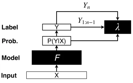
Figure 1: System Overview for SSG. Given an inputX, SSG uses the trained probability to learnλvia a optimizer, which sequentially generates one element of outputYn at a time, given previous outputsY1:n−1, until generating the set of all outputY.
applications (e.g., semantic matching, graph traversal, and question answering), where multiple outputs are required to fully answer a question.
Base Framework: Sequential Set Generation
To handle the variable sizes of the output sets, we split each outputYjinto individual elements and reformulate the train-ing data asD = {( ˆXi,Yˆi) | i = 1, . . . ,Pj|Yj|}, where each Xˆi is an originalXj andYˆi is an element ofYj. For testing, the trained classifier should produce the entire setYkgiven a test sampleXk.
If one directly fits a model between theXˆi’s andYˆi’s, by using, e.g., logistic regression or neural networks, the loss for the same Xˆi = Xj should be similar between the dif-ferentYˆi∈Yj, indicating an equal probability for obtaining one of the correct class labels. These models, however, pro-duce at most one label (subject to any tie breaking mecha-nism) but not the entire set. Rather than developing a new model for our problem, we propose a general framework, called Sequential Set Generation (SSG), that produces a set of labels through leveraging any existing classification mod-els with an additional regularization. The overview of the system is shown in Figure 1.
The proposed framework is suitable for any machine learning classifier and can deal with many different set pre-diction problems. The framework is versatile, and general-izes beyond standard label predictions to, e.g., sequence pre-dictions, where each outputYˆi(an element of the output set Yj), is by itself a sequence. We will discuss the applications of SSG and its generalization to sequence learning.
el-ements sequentially. At each step, we want to find the most plausible answer that has not appeared before, for which we use a memoryZto keep track of. Hence, the predictive out-put is comout-puted as:
Y∗= arg min
ˆ
Y
fθ( ˆX,Yˆ)
s.t. Yˆ 6∈Z,
whereθconsists of the learned parameters of a modelf, and
Zis the set of answers produced so far. To ease computation, we move the constraint to the objective function through La-grange relaxation:
Y∗= arg min
ˆ
Y
fθ( ˆX,Yˆ) +λIXˆ( ˆY ,Z), (1)
whereλis the coefficient for the memory penalty, andI is an indicator function that penalizes a potential label ofXˆ
that has already appeared in the memory Z. One can use the Hamming loss, for example, to computeI:IXˆ( ˆY ,Z) = P
iIXˆ( ˆY =Zi).
In essence, SSG utilizes the memoryZto store existing outputs and repeatedly generates plausible answers to form the output set, until a new answer repeats itself. SSG incor-porates the memory penalty term to realize such a sequential process.
Training and Test for SSG
In what follows, we first consider how SSG works in testing and then state the method for training.
During Testing: Given a query sample Xˆ and a setZ
(which can be either empty or not), Equation (1) produces the next most plausible label. We repeatedly use (1) until a stopping criterion is reached. To ensure all the correct out-put labels are produced, we use the following criterion: if
Y∗in (1) exists inZ, SSG terminates and outputs all the el-ements inZ. Otherwise, SSG storesY∗intoZand compute
anotherY∗. It repeats the procedure to generate correct la-bels while ensuring the incorrect answers are not produced. In the end, the stored memoryZshould contain the entire output set. This testing procedure is summarized in Algo-rithm 1. Note that in order to generate the first element of the set, we use the first term of (1).
This formulation can also answer questions such as “what else would be a good class label given data and existing la-bels.”
During Training: To facilitate the application of different machine learning models, we would like a general training procedure that is widely applicable to different loss func-tions. We have the following training objective:
θ∗, λ∗= arg min
θ,λ L( ˆX, ˆ
Y;θ) +g(λ), (2)
whereL( ˆX,Yˆ;θ)denotes the loss function of a machine learning model, given training data Xˆ = {Xˆi} andYˆ = {Yˆi}, andgis a loss that corresponds to the memory penalty
in (1), which we will elaborate. The functionLmay be any loss (e.g., negative log likelihood) that is associated with the predictive modelfθ.
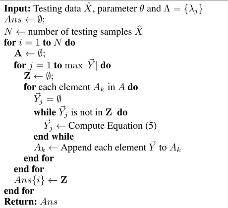
Algorithm 1SSG Algorithm Testing Procedure Input:Testing dataXˆ, parametersθandλ
Z← ∅;Ans← ∅;
N ←number of testing samplesXˆ
fori= 1toNdo
Y∗←arg minYˆfθ( ˆXi,Yˆ) whileY∗is not inZ do
Z←Z∪Y∗
Y∗←Compute Equation (1) end while
Ans{i} ←Z
end for Return:Ans
We observe that the training of the two parameters in (2) can be separated, as the parameter θ for the model f and the memory penalty parameterλresides on different terms. Hence, we first train the first term, equivalent to training any classifier using their specialized procedures (e.g., ran-dom forests, SVM, or neural networks).
Then, we compute the memory penalty coefficientλfrom
g(λ). We would like the memory term to penalize wrong predictions while promoting correct ones. While there ex-ist many choices satisfying this requirement, we use the max-margin principle; i.e., maximizing the gap between the stored labels and other correct labels, as well as those be-tween the stored labels and incorrect labels. We propose the following training objective for robust estimation ofλ:
λ∗= arg min λ
N X
i
[P( ˆYi|Xˆi)−Pˆi−λ]2
s.t. P( ˆYi|Xˆi)−λ≥L−max,Xˆi, ∀i
P( ˆYi|Xˆi)−λ≤L+min,Xˆ
i
, ∀i
whereP( ˆYi|Xˆi)denotes the posterior probability resulting from the trained model,L−
max,Xˆi(resp.
L+
min,Xˆi) is the
max-imal (resp. minmax-imal) posterior probability of the set of neg-ative (resp. positive) labels forXˆi, andPˆiis the average be-tween them; i.e.,Pˆi= (L−max,Xˆ
i
+L+ min,Xˆi
)/2.
The above equation can be solved by using Lagrangian relaxation, leading to:
λ∗= arg min λ
N X
i
||P( ˆYi|Xˆi)−Pˆi−λ||22
−λ+[P( ˆYi|Xˆi)−λ−L−max,Xˆi
]
+λ−[P( ˆYi|Xˆi)−λ−L+min,Xˆi] (3)
whereλ+andλ−are the Lagrangian multipliers of the two
constraints. They can be set to large values to ensure satis-faction of constraints.
Algorithm 2SSG Algorithm Training Procedure Input:Training dataXˆ, training labelsYˆ θ∗←arg minθL( ˆX,Yˆ;θ);
foreach uniqueXˆiinXˆ do Y+←Yˆ[ ˆX
i] ComputeL+
min,Xˆiusing
Y+
Y−←Yˆ\Y+ ComputeL−
max,Xˆiusing
Y− ˆ
Pi ←(L−max,Xˆ
i
+L+ min,Xˆi
)/2
ComputeP( ˆYi|Xˆi)−Pˆi end for
Chooseλ∗from unconstrained minimizer or boundary Return:θ∗, λ∗
on the boundary
min i
n
P( ˆYi|Xˆi)−L−max,Xˆi
o
,
max i
n
P( ˆYi|Xˆi)−L+min,Xˆi o
,
or is equal to the unconstrained minimizer PN
i P( ˆYi|Xˆi)−Pˆi N
if it is feasible, whichever achieves a lower objective value. See Algorithm 2.
After training the model parameter θ, we find the posi-tive label setY+and negative label setY−for each training
dataXˆi. We compute the posterior probabilities for each el-ement ofY+andY−. To follow the max-margin principle, we compute the loss gap for eachXˆiand set the feasible re-gion to be the intersection of all gaps. Finally,λis chosen among the boundary of the feasible region and the uncon-strained minimizer, whichever is feasible and achieves min-imum.
In testing, for eachxi, we first compute the first term of the classification loss, obtaining one labelyij. We then pe-nalize the loss ofyijby computing Equation (2) and attempt to obtain another answeryik, ifyikhas not appeared in the answers. Repeated application of Equation (2) until replica-tion in the answers gives the full set of elements.
Stopping Criterion
The while-loop in Algorithm 1 effectively states that if the computed label is not in the memoryZ, then one should continue producing more. This hard criterion may encounter problems in practice with noisy data. Here, we propose a more robust stopping criterion, which does not affect the be-havior of Algorithm 1 under ideal conditions.
In addition to the memoryZ, we maintain a counterCi indicating the number of times a labelyiis produced. Hence, the predictive function (1) now becomes:
Y∗= arg min
ˆ
Y
fθ( ˆX,Yˆ)+ X
i
Ci·λIXˆ( ˆY =Zi). (4)
What Did You Eat <?> Some Pie Too <?> I Ate Banana <?> I Ate Apple Some Pie Too
I Ate Banana
I Ate Apple
Ans 1:
Ans 2:
Ans 3: <EOS>
<EOS>
λ
<EOS>
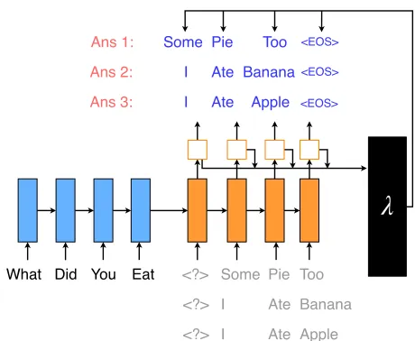
Figure 2: System Overview for SSG-S. Compared with SSG, SSG-S specifically uses a model that can model sequence inputs (such as encoder-decoder networks) to learn the re-lationships and use a optimizer or classifier to learn many differentλ’s.
Let C be the vector of the same dimension as Z. If C
is a vector of all ones, Equation (4) is equivalent to (1). When the elements of C are greater than1, the new cri-terion does not immediately terminate the loop; rather, the loop continues until a certain percentage of the labels have appeared in the memory more than once. In other words, if P
iCi ≥ (1 +ρ)|Z|, whereρis a predefined value with 0 ≤ ρ < 1, Algorithm 1 stops. In a well-trained system, the new stopping criterion will always yield at least one of the true positive labels with a lower objective value than the negative labels. With a judicious choice ofρ, the system be-comes more robust against noise.
Sequential Set Generation for Sequences
The preceding section proposes a method when the output is a set, such as a set of class labels. In many applications, es-pecially natural language problems, however, the elements of the output set are sequences (e.g., sentences), which by themselves are ordered lists comprising sub-elements (e.g., words). In this case, the SSG algorithm proposed so far cannot directly handle sequences, because sequence gen-eration methods (e.g., sequence-to-sequence models (Bah-danau, Cho, and Bengio 2014; Cho et al. 2014)) are iterative and there is no loss associated with the entire sequence. Pe-nalizing the entire sequence with a singleλis not sensible.se-quence, from repeating itself at each location of the output. To achieve so, we need a separateλi for each output loca-tion. LetY~ be one sequence output and letY~ibe an element within the sequence. Given previously generated elements
~
Y1:i−1, we generate the next elementY~ias ~
Yi∗ = arg min ~ Yi
fθ( ˆX, ~Yi|Y~1:i−1) +λiI(Y~i,Zi), (5)
whereZi contains all the i-th elements of the stored out-puts. The first term of (5) is a typical sequence-to-sequence (seq2seq) model, which must be conditioned on the past out-putsY~1:i−1. At each step, it produces a new element given the already produced partial sequence. The second term pe-nalizes the elements that have appeared in the stored output. For each location of the sequence, the penalty is different.
Similar to the preceding section, the model parameterθ
and the penalty parametersΛ = {λi}are trained by using the objective
θ∗,Λ∗= arg min
θ,Λ L( ˆX,
ˆ
Y;θ) +g(Λ),
where( ˆX,Yˆ)denotes the training data and L is any loss in a seq2seq model that comes with the predictive function
fθ in (5). The training ofθ is standard. The second term g(Λ)is used to train the penalty parametersΛ = {λi}. For each locationiin the output sequence,λiis trained by using, again, the max-margin principle through
λ∗i = arg min λi
N X
j
[P(Y~j,i|Xˆj, ~Yj,1:i−1)−Pˆj,i−λi]2
s.t. P(Y~j,i|Xˆj, ~Yj,1:i−1)−λi≥L− max,Xˆj,i
, ∀j
P(Y~j,i|Xˆj, ~Yj,1:i−1)−λi≤L+min,Xˆj,i,
∀j.
The solution is similar to that in the preceding section, for eachi.
The training and testing algorithms are shown in Algo-rithms 3 and 4, respectively. The training of SSG-G is sim-ilar to SSG, and the only difference is that theλ’s are com-puted for each token level in a sequence, resulting in a total of max|Y~|number of λ. The notationmax|Y~|represents the maximal allowable sequence length in any of the out-puts.
SSG-S has noticeable differences in testing from SSG. Specifically, SSG-S does not generate one sequence in its entirety before generating the next one. On the contrary, it generates all possible answers for each position in a se-quence. This approach allows efficient data structures if de-sired, such as a Trie-tree, to keep track of all the sequences in the set, although it is also capable of sequentially pro-ducing one sequence at a time. For each inputxiand at each output positionj, SSG-S monitors the generated setAof se-quences so far (each with a lengthj−1). For each sequence
AkinA, SSG-S generates all possible tokensY~jat position j by repeatedly finding the most probable solution and pe-nalizing it. In other words, the testing procedure is similar to that of SSG, except for the explicit consideration of all the partial sequenceAk. Then, SSG-S appends each token inY~j
Algorithm 3SSG-S Algorithm Training Procedure Input:Training dataXˆ, training sequencesYˆ θ∗←arg minθL( ˆX,Yˆ;θ);
foreach uniqueXˆiinXˆ do Y+←Yˆ[ ˆX
i] Y−←Yˆ\Y+
for j= 1tomax|Y~| do
ComputeL+
min,Xˆi,j using
Y+
ComputeL− max,Xˆi,j
usingY− ˆ
Pi,j←(L−max,Xˆ
i,j
+L+ min,Xˆi,j
)/2
ComputeP( ˆYi,j|Xˆi, ~Yi,1:j−1)−Pˆi,j end for
end for
for j = 1tomax|Y~| do
Chooseλ∗j from unconstrained minimizer or boundary end for
Return:θ∗,{λ∗j}
to the correspondingAk, producing new sequencesAkwith lengthj. Note that the previously generated answers inAk are used as context in the overall generation process. It can be achieved by feedingAk into the decoder as input for the next token, a procedure similar to “teacher forcing” in train-ing seq2seq. With this gradual expansion of the answer set
A, SSG-S produces all the feasible sequences.
Deep Sequential Set Generation
While SSG-S handles short sequences quite well, in prac-tice data can be unbalanced and have increasing complexity for long sequences and large vocabulary. The loss for dif-ferent correct outputs in a set can hence substantially differ, depending on the label frequencies at each position of the se-quence. This phenomenon could lead to a problem that one singleλ, or even a fixed set ofλ’s, cannot distinguish the positive and negative sets in different contexts. To remedy this difficulty, we introduce a deep learning-based approach to distinguish the positive classes from the negative ones at each position j in the sequence, replacing the learning of allλ’s as discussed in the preceding section. In essence, we use a neural network to classify positive and negative tokens in the sequence. Specifically, we still train a seq2seq model as discussed previously. However, now we feed the loss se-quence in the final output layer into another neural network, which we call theλ-network.λ-network classifies each pos-sible label from the original network into either positive or negative class at that token value. During training, the λ -network is learned by taking the loss from the decoder logits as inputs, and produces a binary label (indicating whether each label is a positive class) at positionj. We consider both recurrent neural networks (RNN) and convolutional neural networks (CNN) as the classifier. Their structures are shown in Figure 3.
P1
P2
Pk
... <?> ... ...
y0
y1
yk
y0
y1
Encoder Decoder
RNN Optimizer
a)
Conv1D MaxPool Dense Dense Sigmoid
CNN Optimizer
b)
[ID, k, , , . . . ]P1 P2 Pk
yk
ID
Figure 3: Architectures of RNN and CNNλ-Optimizer, as a part of SSG-S. Instead of learningλ’s directly, a neural-network-based classifier is used. Subfigure(a)shows the RNN architecture, and(b)shows the CNN architecture used in the experiments.
Algorithm 4SSG-S Algorithm Testing Procedure Input:Testing dataXˆ, parameterθandΛ ={λj} Ans← ∅;
N ←number of testing samplesXˆ
fori= 1toNdo
A← ∅;
forj= 1tomax|Y~|do
Z← ∅;
foreach elementAkinAdo ~
Yj =∅
whileY~jis not inZ do ~
Yj ←Compute Equation (5) end while
Ak←Append each elementY~ toAk end for
end for
Ans{i} ←Z
end for Return:Ans
target sequence as an input to the encoder part of the RNN, and then use the binary labels on each logit as training target for the decoder. For the CNNλ-optimizer, we feed decoder logits and the position IDj as well as the logit ID k, and use one 1D-convolution and max pooling layers, multiple densely connected layers, and one sigmoid layer. The output of CNN is the binary label ofk-th element of the logit. Note that theλ-network only replaces the learning ofλin Algo-rithm 3 and Equation (5) of AlgoAlgo-rithm 4. The rest of the training and testing algorithms remain unchanged. We call the methods respectively SSG-RNN and SSG-CNN. Note that SSG-S along with SSG-RNN and SSG-CNN can both be used for the singleton sets, which can be considered as sequences of length 1.
Experiments
We conduct experiments to evaluate the proposed algorithms on various applications, comparing against existing base-lines if possible.
Benchmark Dataset
While it is not the intended application of the proposed se-quential set generation algorithms, SSG can be applied to label problems. We compare SSG with standard multi-label techniques on the YEAST and SCENE dataset, both of which are publicly available. YEAST is in the domain of bi-ology. It contains over2000data samples and has the feature size of103. The unique label number is14, and the average cardinality is4.2. The SCENE data has2407samples,294
features, and6unique labels.
We compare with the standard sigmoid network (Grodz-icki, Ma´ndziuk, and Wang 2008), where each possible la-bel is considered as a binary classification problem. For fair comparison, we use the same base architecture for both the sigmoid network and deep SSG models, and take the sig-moid output as the input to λ-optimizer in SSG. Since the baseline consists of deep models, we only compare deep ver-sions of SSG. We do a train-test split of70−30, and use the standardF1score to measure the accuracy performance of different methods. We then take the mean,mF1, as the ac-curacy score to compare the ground truth label set and the learned set. The higher themF1score, the better.
Table 1: MeanF1Accuracy Result on Benchmark Dataset of Various Algorithms. SSG-CNN shows the best performance.
Multi-Label SSG-RNN SSG-CNN
YEAST 0.430 0.402 0.658
Table 2: Experiment Accuracy Results of Various Algorithms on Two Complex Reasoning Tasks involving Set Output and Set of Sequences.
MeanF1score (mF1) and mean Edit Distance (mED) are Used.
Metric Multi-Label SSG-S SSG-RNN SSG-CNN
Task 1 mF1, the higher the better 0.64 0.19 0.42 0.70 Task 2 mED, the lower the better N/A 8.10 3.75 2.00
As one can see from Table 1, SSG substantially outper-forms the simple sigmoid network for multi-label classifi-cation. Although one might use different or more complex architectures than the sigmoid network, we believe the rel-ative improvement would be consistent (which supported in the following more complex tasks).
Synthetic Datasets
We conduct two experiments to compare the proposed meth-ods: a number problem that predicts sets, and another prob-lem that predicts a set of sequences. We first describe each problem, with the aim of tackling complex reasoning tasks that traditional machine learning methods cannot handle. Task 1: Predicting Sets. In this task, the input is a positive integer read as a string of digits. Let the leading digit be
m. The output is the set of m leading digits of the input string, with duplicates counted only once. For example, if
X = 33874, thenY ={3,8}. We call this Task-1. We again usemF1as the accuracy score to compare the ground truth label set and the learned set.
Task 2: Predicting Set of Sequences. In the second task, the input is a digit string of length 20. Let the string be evenly split into two halves. The first 10 digits are grouped into five pairs:(s1, e1), . . . ,(s5, e5); and the last 10 digits constitute a string a. The output set consists of (at most) 5 subsequences of a: a[s1, e1), . . . , a[s5, e5). Whenever
si ≥ ei for some i, the substring is empty and hence it does not count as an element of the output set. Similar to the first data set, duplicate strings are removed. For exam-ple, ifX = 00490000349172105519, thenY ={2,10551}. The elements ofY are substringsa[4,9)anda[3,4), where
a = 9172105519. Note that 0-based indexing is used here. Treated as a multi-label classification problem, the number of classes is1010, which is impossible to handle. We call this Task-2. We use mean edit distance, mED, as the ac-curacy score to compare the ground truth set of sequences and the learned set of sequences. For ground truth set and learned set, we compute ED distance between every pair of sequences and divided by the total number of pairs. The lower the scoremED, the better.
System Architecture: Since both tasks have sequence in-puts, we use an encoder-decoder architecture (Sutskever, Vinyals, and Le 2014b). We use a one layer LSTM with60
encoder hidden units and120decoder hidden units. An em-bedding layer of size60is used for appropriate discrete in-puts and outin-puts. We use Adam optimizer (Kingma and Ba 2014) with a batch size of15, and cross entropy as loss func-tion. We generate 1000 samples and randomly split70%as training and the rest as testing.
We compare three methods S, RNN, and SSG-CNN with the baseline multi-label sigmoid network for these two tasks. Table 2 shows the results. In both tasks, we can see that SSG-CNN is the best method, outperforming the second best SSG-RNN by a large margin (28% mF1
and 1.75mED). Moreover, the neural-network-based SSG-CNN and -RNN outperform SSG-S, showing that it is very important to consider the complexity of reasoning tasks. Note that we did not tune or search for the best hyper-parameters and it is reasonable to assume that these perfor-mance figures can be further improved. SSG-CNN also out-performs the multi-label method on Task 1, and the multi-label method is not applicable to Task2due to the extreme modeling complexity.
Conclusion
We proposed a general framework, SSG, along with three variants, designed to solve set-valued output problems. We developed a sequential generation approach that can effi-ciently learn set relationships from data, as demonstrated on benchmark and reasoning tasks. Experiments show that the sequential generation procedure can improve performance on traditional multi-label tasks and can handle more com-plex sets such as set of sequences, where traditional methods are not readily applicable.
Further work will include theoretical analysis on the rela-tionships between the set size and the learning performance, investigation on better training methods for SSG, and testing on a wider variety of set components, including sets of sets. We believe set-valued outputs have many applications such as theorem proving in AI and are foundational for systems that perform reasoning in particular, making their general treatment an important research direction to address.
Acknowledgments
We thank for colleagues at AISR for helpful discussion and anonymous reviewers for insightful comments.
References
Argyriou, A.; Evgeniou, T.; and Pontil, M. 2007. Multi-task feature learning. InAdvances in neural information process-ing systems, 41–48.
Argyriou, A.; Evgeniou, T.; and Pontil, M. 2008. Convex multi-task feature learning. Machine Learning73(3):243– 272.
Bahdanau, D.; Cho, K.; and Bengio, Y. 2014. Neural ma-chine translation by jointly learning to align and translate.
Cho, K.; van Merrienboer, B.; G¨ulc¸ehre, C¸ .; Bougares, F.; Schwenk, H.; and Bengio, Y. 2014. Learning phrase rep-resentations using RNN encoder-decoder for statistical ma-chine translation.CoRRabs/1406.1078.
Grodzicki, R.; Ma´ndziuk, J.; and Wang, L. 2008. Improved multilabel classification with neural networks. In Interna-tional Conference on Parallel Problem Solving from Nature, 409–416. Springer.
Hinton, G.; Deng, L.; Yu, D.; Dahl, G.; rahman Mo-hamed, A.; Jaitly, N.; Senior, A.; Vanhoucke, V.; Nguyen, P.; Sainath, T.; and Kingsbury, B. 2012. Deep neural net-works for acoustic modeling in speech recognition. Signal Processing Magazine.
Irving, G.; Szegedy, C.; Alemi, A. A.; E´en, N.; Chollet, F.; and Urban, J. 2016. Deepmath-deep sequence models for premise selection. InAdvances in Neural Information Pro-cessing Systems, 2235–2243.
Kingma, D. P., and Ba, J. 2014. Adam: A method for stochastic optimization.arXiv preprint arXiv:1412.6980. Sutskever, I.; Vinyals, O.; and Le, Q. V. 2014a. Se-quence to seSe-quence learning with neural networks. CoRR
abs/1409.3215.
Sutskever, I.; Vinyals, O.; and Le, Q. V. 2014b. Sequence to sequence learning with neural networks. InAdvances in neural information processing systems, 3104–3112. Taskar, B.; Chatalbashev, V.; Koller, D.; and Guestrin, C. 2005. Learning structured prediction models: A large mar-gin approach. InProceedings of the 22nd international con-ference on Machine learning, 896–903. ACM.
Tsoumakas, G.; Katakis, I.; and Vlahavas, I. 2009. Mining multi-label data. InData mining and knowledge discovery handbook. Springer. 667–685.
Vinyals, O.; Bengio, S.; and Kudlur, M. 2016. Order mat-ters: Sequence to sequence for sets. InInternational Confer-ence on Learning Representations (ICLR).
Vinyals, O.; Toshev, A.; Bengio, S.; and Erhan, D. 2014. Show and tell: A neural image caption generator. CoRR
abs/1411.4555.
Xue, Y.; Liao, X.; Carin, L.; and Krishnapuram, B. 2007. Multi-task learning for classification with dirichlet process priors. Journal of Machine Learning Research8(Jan):35– 63.
Zaheer, M.; Kottur, S.; Ravanbakhsh, S.; Poczos, B.; Salakhutdinov, R. R.; and Smola, A. J. 2017. Deep sets. In
Advances in Neural Information Processing Systems, 3394– 3404.