R E S E A R C H
Open Access
Multi-candidate missing data imputation for
robust speech recognition
Yujun Wang
*and Hugo Van hamme
Abstract
The application of Missing Data Techniques (MDT) to increase the noise robustness of HMM/GMM-based large vocabulary speech recognizers is hampered by a large computational burden. The likelihood evaluations imply solving many constrained least squares (CLSQ) optimization problems. As an alternative, researchers have proposed frontend MDT or have made oversimplifying independence assumptions for the backend acoustic model. In this article, we propose a fast Multi-Candidate (MC) approach that solves the per-Gaussian CLSQ problems
approximately by selecting the best from a small set of candidate solutions, which are generated as the MDT solutions on a reduced set of cluster Gaussians. Experiments show that the MC MDT runs equally fast as the uncompensated recognizer while achieving the accuracy of the full backend optimization approach. The
experiments also show that exploiting the more accurate acoustic model of the backend does pay off in terms of accuracy when compared to frontend MDT.
Keywords:speech recognition, constrained optimization, missing data, noise robustness
1. Introduction
One of the major concerns in deploying Automatic Speech Recognition (ASR) applications is the lack of robustness of the technology when compared to human listeners. A key aspect is the sensitivity to background noise. This effect is caused by the differences between the conditions in which the statistical models for speech are trained and those in which they are applied in real-life situations. Many approaches which reduce the mismatch to improve the noise robustness of speech recognition have been proposed earlier. They modify either the frontend signal preprocessing or the backend acoustic model of the recognizer. A popular frontend method is the Advanced Front-End [1] which applies multiple stages of Wiener filtering to remove the back-ground noise from the corrupted observations. Other techniques working in the frontend are, e.g., spectral subtraction [2], Stereo Piecewise Linear Compensation for Environment [3] and the Vector Taylor series com-pensation algorithm [4]. Some examples of backend approaches are Parallel Model Combination (PMC) [5] and model adaption algorithms, such as Maximum
Likelihood Linear Regression (MLLR) [6] and Maximum A Posterior probability (MAP) based adaptation [7].
In the late 1990s, Missing Data Techniques (MDT) were introduced in speech recognition as a perceptually moti-vated approach to improve the noise robustness of a speech recognizer. Research in Auditory Scene Analysis (ASA) [8] proposed models for the capability of human listeners to deal with concurrent signals. The human audi-tory system is able to extract sufficient information from the speech source of interest in order to recognize what is said, even if parts of the target signal are masked by other signals. It exploits the redundancy in the speech signal and can thus handle missing data. The motivation of MDT is to explore these capabilities of human listeners and exploit them in ASR to reduce the performance gap between humans and computers. It relies on the model that a given spectral band at a given time is dominated by either speech or noise. In the frontend preprocessing, the time-frequency regions of a speech signal are labeled as reliable or as unreliable. This labeling information is encoded into a so-calledmissing data mask. In the backend decoding, features in the unreliable regions are either ignored or pre-dicted to alleviate the mismatch. This compensation strat-egy relies only on the speech model and unlike PMC for instance, it does not require a model of the noise, though * Correspondence: [email protected]
Department of ESAT, Katholieke Universiteit Leuven, Kasteelpark Arenberg 10, B-3001 Leuven, Belgium
some assumptions about the noise are required instead while generating the missing data mask [9,10]. In recent years, the MDT was extended to techniques such as the glimpsing model [11] and speech fragment decoding [12]. Other related work includes the propagation of uncer-tainty [13] where the authors transform the unceruncer-tainty encoded in the binary mask from the spectral domain to the cepstral domain, and handle the transformed uncer-tainty with the cepstral backend acoustic models. The authors of [14] introduce a two-pass MDT system, where the lattice generated by the MDT recognizer in the first pass is rescored. In the second pass, a state-based hypoth-esis test then generates the so-called“integrated mask”, yielding better recognition results.
The two major problems in MDT are first estimating the mask and then exploiting these masks during recog-nition. Identifying the‘missing’part during recognition is an essential step in MDT as proposed by Cooke et al. [15] and Lippmann and Carlson [16]. A missing data detector makes a binary decision about which spectro-temporal components are unreliable due to noise distor-tions and which remain reliable, i.e., are dominated by speech. Approaches of missing data mask estimation, such as Bayesian classification [17], harmonic mask esti-mation [10], local SNR-based mask estiesti-mation [18,19], and VQ mask estimation [9] mainly exploit characteris-tics of the speech signal. The authors of [20] estimate the missing data masks based on computational ASA. More approaches can be found in a survey on missing data mask estimation by Cerisara et al. [21]. The concept of binary reliability masks can be extended tosoft masks [22] when uncertainty about the reliability information is taken into account. The mask then assumes continuous values instead of binary values. Soft masks are not con-sidered in this article, as we have found them to provide little benefit in [23].
Several paradigms have been designed to apply MDT once the masks are computed. MDT was first formulated for a spectral acoustic model [15], which is referred to as spectral MDTin this article. The spectral energy within each unreliable component can be either reconstructed based on the acoustic model and the reliable information, or marginalized out of the probability density functions (PDF) of the HMM states. The former scheme is defined asimputationand the latter is defined as marginaliza-tion. In order to improve the performance of MDT, Raj et al. [24], Van hamme [25], Cerisara [26], Häkkinen and Haverinen [27], and Faubel et al. [28] applied MDT using cepstral acoustic models, which are referred to ascepstral MDTin this article. The experimental results of cepstral MDT demonstrate its advantage over the spectral model. The authors of [24] used MDT imputation to enhance the speech features in the front-end, while in Maximum Likelihood (ML) Gaussian-based imputation [25] and in
conditional mean imputation [28], the authors consider MDT imputation associated with Gaussians in the backend.
The above work addresses the robustness of the MDT system rather than its efficiency. MDT systems involve much more intensive computation in the backend, as explained in Section 3. This was already noticed in [15], where the problem was addressed by compromising on the acoustic model (diagonal Gaussians for log-spectral features). An alternative solution is to formulate MDT as a front-end technique [24]. In this article, we propose a Multi-Candidate (MC) MDT which not only produces competitive recognition accuracy, but also possesses the same efficiency as a conventional large vocabulary recog-nizer under noisy conditions. We advocate the backend approach, since it exploits the most accurate speech model that is available in the recognizer to compensate for the missing data. Each HMM state represents an accurate hypothesis about what the missing speech could be, integrating all knowledge that is available in the deco-der: acoustics, lexical information, and language model. Hence, we expect more accurate missing data imputation than with frontend MDT approaches, where such sophis-tication is not available. In our setting, we go beyond the state level and compute a clean speech vector per Gaus-sian. In addition to the entire set of Gaussians embedded in the HMM, a fairly small set of Gaussians are trained to function as cluster Gaussians (CG). They provide feasible candidates (i.e., they satisfy the constraints for the imputed data, as described in Section 2.1) of imputations for the entire set of Gaussians. As such, instead of solving the full optimization problem for each Gaussian in the acoustic model, candidate solutions are selected from the CG and the most likely one is retained. Therefore, imple-mentation of MC MDT requires only a modest modifica-tion of convenmodifica-tional HMM-based recognizers. The MC MDT forms the main contribution of this article. It is an algorithm that aims at computational gains for large vocabulary speech recognizers without sacrificing accuracy or robustness. It provides a solution for applying MDT to an existing backend model trained for the speech feature vector of one’s choice. Furthermore, we show experimen-tally that we gain more immunity to noise than if MDT is applied as a frontend feature-enhancement technique [24] and compare several methods for solving the impu-tation problem.
framework of ML decoding and why it becomes difficult when using a model trained with decorrelated features such as cepstral features or features generated by, e.g., linear discriminant analysis (LDA) [29]. Section 4 describes the approach of MC MDT imputation using CG to speed up the Gaussian-based imputation. Section 5 explains how to further speed up the imputation of the CG by selecting a subset of the CG dynamically. Section 6 describes several experimental results. Finally, in Sec-tion 7 we present our conclusions and propose future work.
2. Spectral and Cepstral MDT systems
In this section, we review some of the concepts of MDT that lead to approaches that are most related to the pro-posed system.
2.1. Bounds
Environmental noises are assumed to be additive in the spectral domain. Hence, at framet, the log-spectra of the underlying complete clean speechxtcan be assumed to be approximately bounded above by the observed noisy feature vectoryt, namely:
xt≤yt (1)
where the inequality sign for vectors applies compo-nent-wise. Both xtandytcan be partitioned into their reliable and unreliable sub-vectors according to the mask:
xt=
xt,r xt,u
andyt=
yt,r yt,u
For the reliable spectro-temporal regions, the observed noisy features are deemed to be pure speech:
xt,r=yt,r,
whereas for the unreliable regions, the observed fea-tures act merely as upper bounds for the clean speech:
xt,u≤yt,u
2.2. State-based imputation and marginalization
The authors of [15] formulated several MDT approaches which use the acoustic models trained in the same domain in which the masks are expressed and in which the con-straints of Equation (1) hold. In their experiments, the acoustic feature vectors are obtained via a 64-channel auditory filter bank with center frequencies spaced linearly on an ERB scale from 50 Hz to 8 kHz. The HMM-based speech recognizer is adapted to accommodate MDT by modifying the state likelihood evaluation as outlined below. Each HMM state is expressed as a mixture of mul-tivariate Gaussians with a diagonal covariance matrix. The MDT here is carried out frame-by-frame and is assumed independent across frames. The authors proposed both state-based imputation and marginalization. Besides the upper boundyt, u, a lower bound can also be applied to
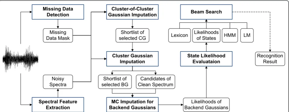
Cluster-of-Cluster Gaussian Imputation
Cluster Gaussian Imputation
MC Imputation for Backend Gaussians Missing Data
Detection
Spectral Feature Extraction
Missing Data Mask
Noisy Spectra
Shortlist of selected CG
Candidates of Clean Spectrum Shortlist of
selected BG
Likelihoods of Backend Gaussians
State Likelihood Evaluataion Beam Search
Likelihoods of States
Recognition Result HMM
Lexicon LM
control the arbitrariness of compensation for the unreli-able components. This idea can be applied to all methods described in this article. However, for consistency, we will omit lower bounds from this article.
In state-based marginalization, each state output PDF is a function of the reliable components only, while the unreliable components are marginalized out, i.e., each unreliable component is integrated over the range of values it can assume. The PDF of a statesis given by:
p(yt,r|s) =P(k|s)
k∈G (s)
p(yt,r|k,s)
yt,u
−∞p(xt,u|k,s)dxt,u
whereG(s) represents the set of Gaussians belonging to the Gaussian Mixture Model (GMM) of states. The integral of Gaussian kcan be calculated using the com-ponent-wise error function because its covariance matrix is assumed to be diagonal.
In state-based imputation, the clean speech is imputed for every state s, followed by calculating the likelihoods using the imputed values, which will be utilized to expand hypotheses in the search space during decoding. Two ways of imputing the clean speech per state are given: linear combination or winner-takes-all.
In linear combination, the Minimum Mean Squar Error (MMSE) estimate of the imputation from statesis
ˆ
xt,u,s= k∈G(s)
P(k|yt,r,s)µu,k
where μu, k is the unreliable sub-vector of mean of Gaussiankand
P(k|yt,r,s) =
P(k|s)p(yt,r|k)yt,u
−∞p(xt,u|k)dxt,u
j∈G(s)
P(j|s)p(yt,r|j)yt,u
−∞p(xt,u|j)dxt,u
In winner-takes-all, after the clean speech is imputed for each Gaussian belonging to states, the mixture’s like-lihood is evaluated for all imputed values and the most likely imputation is selected as the imputation of the state. In other words, the imputation of statesis approxi-mated by the clean speech vector imputed from its kˆ th member Gaussian:
ˆ
xt,u,s∼= xˆt,u,ˆk
where kˆ= arg max
k∈G(s)
p(xˆt,u,k|s). xt,u,k is the maximum
likelihood imputation of the unreliable subsectorxt, u, k for Gaussiankincluded in G(s):
ˆ
xt,u,k= arg max
xt,u,k≤yt,u
p(xt,u,k|k) k∈G (s)
This problem has a closed form solution:
ˆ
xt,u,k= µu,k
ifµu,k≤yt,u
yt,u ifµu,k>yt,u k∈G (s) (2)
where it should be understood that we have written the solution vectorially for convenience, but the top or bottom case in (2) may apply to different vector compo-nents. The imputation using a spectral acoustic model containing Gaussians with a diagonal covariance matrix has an analytical solution because the components of the log-spectral features are considered to be indepen-dent. However, the spectral features do have correlation among their components and the spectral GMM used above is not very effective to model this. The perfor-mance of HMM speech recognizers using GMMs with diagonal covariance is significantly better when using decorrelated features, e.g., MEL Frequency Cepstral Coefficients (MFCC). Therefore, a cepstral MDT model with diagonal covariance-Gaussians is introduced in the following section.
2.3. Spectral reconstruction
In [24], the authors reconstruct the spectral features using either a correlation-based method or a cluster-based method. The reconstructed spectra are then trans-formed into cepstra for processing by the speech recognizer.
The correlation-based approach solves the imputation of unreliable components at each frame by exploiting the correlations among the components in the spectro-temporal representation. The correlation is modeled by a Gaussian wide-sense stationary (WSS) process whose parameters are learned from training data. The core of the algorithm is a bounded MAP estimate:
ˆ
xt,u= arg max
xt,u≤yt,u
p(xt,u|yt,n) (3)
whereyt, nis the neighborhood vector containing all the related reliable components which are spectrally and temporally sufficiently close to xt, u as defined by the WSS model. The likelihoodp(xt, u|yt, n) is modeled with a full covariance Gaussian conditioned on the observed yt, n. The authors establish an iterative approach to solve (3).
ˆ
xt,u= M m=1
P(mxt,u,m≤yt,u,yt,r)xˆt,u,m (4)
where
ˆ
xt,u,m= arg max
xt,u,m≤yt,u
p(xt,u,m|yt,r,m) (5)
is the imputation resulting from the mth CG, a bounded optimization problem which can be solved by the MAP algorithm as in the correlation-based approach. P(m|xt, u, m ≤ yt, u , yt, r) is the posterior probability of the CG given the reliable data and the fea-sible region for the unreliable data.
P(mxt,u,m≤yt,u,yt,r) =
P(m)yt,u
−∞P(xt,u,m,yt,r|m)dxt,u,m M
j=1
P(j)yt,u
−∞p(xt,u,j,yt,rj)dxt,u,j
(6)
To make computation of this posterior probability tractable, the spectral CGs are assumed to be diagonal in this circumstance.
In both the correlation-based and the cluster-based method, the reconstruction is separated from the decod-ing and there is only one sdecod-ingle imputation per frame, while in the spectral state-based imputation of Section 2.2, each state or Gaussian has its own imputation, which is theoretically more suitable for an ML-based recognizer. The likelihood of each state is calculated at its imputed value and used in the backend of the recog-nizer which incorporates the lexical and grammatical knowledge to drive the path pruning in the beam.
It should be noted that the authors of [15] show that state-based marginalization outperforms state-based imputation. Therefore, it would be natural to formulate marginalization for cepstral or other decorrelated mod-els as well. However, this leads to definite integration of full covariance Gaussians. Even if approximations described in [28] would be applied to marginalization, the computational complexity is not acceptable for a practical speech recognizer. Hence, we only focus on imputation with decorrelated models.
3. Missing data imputation for maximum likelihood decoding
State-of-the-art automatic speech recognizers take a Bayesian approach, i.e., the decoding process is to find a sequence of words Wˆ whose posterior probability is maximal given aT-frame sequence of observationsy1...T:
ˆ
W= arg max
W
P(W|y1···T)≈arg max
W
p(y1···T|s1···T)P(W)
where the language modelP(W) is the probability of a hypothesized word sequence W. In practice, the most
likely state sequence s1...T that realizes W is found. In MDT, the maximization should be additionally taken over the unreliable features to be imputed, i.e.,x1...T, u, to find out the optimal imputation xˆ1...T,u bounded by
the noisy observationy1...T, u.
(Wˆ,xˆ1...T,u) = arg max
W,x1...T,u≤y1...T,u
p(x1···T,u,y1...T,r|s1···T)P(W).
For a given state sequences1...TwithWembedded, the complete speech is given by the following expression, where we have assumed state-conditional independence ofx1...T, u:
ˆ
xs1...T,u= arg max
x1...T,u≤y1...T,u
p(x1···T,u,y1...T,r|s1···T) =a T
t=1
arg max xt,u≤yt,u
p(xt,u,yt,r|st) (7)
wherea is the product of the transition probabilities between the states on the hypothesized path. The maxi-mization in Equation (7) can be accomplished frame-by-frame, i.e., the optimal clean speech at timetis obtained by the maximization of the output PDF of state s over the complete speechxtbounded by the observationyt:
ˆ
xt,u,s= arg max xt,u,s≤yt,u
p(xt,u,s,yt,r|s) = arg max xt,u,s≤yt,u
k∈G(s)
P(k|s)p(xt,u,s,yt,r|k) (8)
Equation (8) formulates an ML state-based missing data imputation. The constrained optimization in (8) is not computationally tractable. If each member Gaussian in a state output PDF is assumed to impute its own clean speech using MLE:
ˆ
xt,u,k= arg max
xt,u,k≤yt,u
p(xt,u,k,yt,r|k) (9)
MDT imputation becomes ML Gaussian-based impu-tation, which is an approximation of the state-based imputation but is computationally more tractable. It will be shown in Section 6.4.4 that (8) and (9) yield compar-able recognition accuracy.
If the model used for imputation is trained with ceps-tral features or other decorrelated features, such as LDA [29] or HLDA [30] features, Gaussiank can be formu-lated in the log-spectral domain after the corresponding linear transformationCof full row-rank is applied:
p(xt,k|k) = 1
(2π)Dm|
k| exp
−1
2(Cxt,k−µk)
k−1(Cxt,k−µk)
= 1
(2π)Dm|
k| exp
−1 2(xt,k−C
+µ
k)Ck−1C(xt,k−C+µk)
Qk= (xt,k−C+µk)Ck−1C(xt,k-C+µk) (10)
with the precision matrix
Hk=Ck−1C
the maximization of (9) overxt, kbecomes:
ˆ
xt,u,k= arg min
xt,u,k≤yt,u
xt,u,k
yt,r
−C+µ
k
Hk
xt,u,k
yt,r
−C+µ
k
(11)
Notice thatHkcan be singular (e.g., when the cepstral features have less dimension than the log-spectral fea-tures), in which case ak-dependent small fraction of the identity matrix is added to regularizeHk, so a unique solu-tion of (11) is found. Since Hk is not diagonal, the bounded minimization in (11) can no longer be solved by Equation (2). Instead, it becomes a Constrained Least Square (CLSQ) problem, which does not have an analyti-cal solution. Methods such as the MAP algorithm [24], primal active set methods [31], Multiplicative Updates (MU) [32], and imputation with PROSPECT features [33] have been proposed. But, their computational cost for large vocabulary speech recognizers with tens or hundreds of thousands of Gaussians becomes prohibitive. Below, the MC MDT imputation is proposed to significantly reduce the computational intensity to achieve an MDT recognizer with speed.
4. MC missing data imputation
In (11), Gaussian-based imputation is formulated as searching for the optimal clean speech vector within a fea-sible region, i.e., the (continuous) subspace which is spanned by the unreliable components and is bounded by the observation. This process can be approximated by evaluating each Gaussian on a list of feasible clean speech candidates and then selecting the candidate which maxi-mizes the likelihood as the imputed value. This approxi-mation is the basic idea behind the MC MDT imputation. For every Gaussian, the list of candidates is given by the imputation from a small set of CG. The Gaussians in the acoustic model, typically a large number, will be called BGs in the remainder of the article. The optimization for each BG in (11) is then approximated by selecting the
ˆlt,kth clean speech candidate such that:
ˆlt,k= arg max l∈k p
˜
xt,u,l,yt,rk
,i.e.xˆt,u,k∼= x˜t,u,ˆlt,k (12)
whereΩkrepresents all the CGs which might generate suitable solutions for Gaussiank, and x˜t,u,l is the clean
speech estimate of the unreliable speech components obtained from CG l. The construction of Ωk will be detailed in Section 4.3. Hence, in MC MDT, solving the CLSQ problem of BG k is replaced by Lk likelihood
evaluations, whereLk is the cardinality ofΩk. Whereas solving a large number of BG imputation problems is avoided, the task is shifted to the restricted set of CGs. Solving each of these problems requires a computational effort that is at least an order of magnitude greater than the evaluation of a Gaussian likelihood, so various approaches for the imputation with CGs are discussed below.
4.1. ML-imputation for CG
The imputed value from the CGs can be computed by iterative approaches such as Gradient Descent (GD) [33], MU [32], or MAP [24]. In GD, the gradient for iterationτis
gt,kτ =Hk(xt,kτ−1−C+µk)
where each negative component ofgt, kτ, for whichxt,
kis on the boundaryyt, is zeroed and so is each reliable component of gt, kτ in order to not violate the con-straints. Since the cost function in Equation (10) is quadratic, the optimal step for iterationτ has an analytic expression:
stept,kτ =
−(gt,kτ)gt,kτ
(gt,kτ)Hkgt,kτ
gt,kτ (13)
The step direction is maintained, but the step size is reduced such that the boundary constraints are not vio-lated.
xt,kτ=xt,kτ−1+stept,kτ xt,kτ ≤yt
To initialize the GD algorithm, the non-diagonal cov-ariance structure is ignored, i.e., it starts from the solu-tion in Equasolu-tion (2).
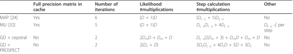
We opt for GD rather than MU [32] or MAP [24] because it benefits from several advantages simulta-neously: (i) the number of iterations required for practi-cal convergence is smaller [33], (ii) the gradient computation (13) can be carried out from right to left such that only a small number of matrix-vector multipli-cations and vector operations are required (see Appen-dix), (iii) only theconstant transformation matrixC, the observation, mean, and variances need to be copied to the cache memory of the CPU while other methods may require a larger memory access bandwidth, (iv) GD does not require square root operations like MU, hence the total number of arithmetic operations per iteration is less than that of MU (as shown in Table 1).
The computational effort is further reduced by using PROSPECT features together with GD, which is pro-posed in [33].
Dc= 4), which models the rough shape of the spectrum at timet. This cepstral part is given by
vct =Ccxt
where Cc denotes the reduced DCT matrix with orthonormal rows. The remaining details of the signal are captured by
v⊥t = (I−CcCc)xt
which is termed the projection part because it is the orthogonal projection of xton the orthogonal comple-ment of the subspace spanned by the rows of Cc. The concatenation of the cepstral part and the projection part is referred to as PROjected SPECTral (PROSPECT) features:
vt =
vc t v⊥t
=Rxt
The PROSPECT transformation matrix is
R=
Cc
(I−CcCc)
The likelihood of thekth Gaussian based on the PRO-SPECT features is formulated as
F(vt|k) =p(vct|k)p(v⊥t |k)β (14)
where
p(vc t|k) =
1
(2π)Dcc
k
exp
−1
2(v
c t−µck)ck
−1
(vc t−µck)
(15)
and
p(v⊥t|k) = 1 (2π)D⊥k
exp
−1
2(v
⊥ t −µ⊥k)⊥k
−1
(v⊥t −µ⊥ k)
(16)
where µck, ck, µ⊥k, and ⊥k are the means and cov-ariance matrices of cepstral and projection part of PRO-SPECT Gaussiank, respectively. They are all estimated
on data using the EM-algorithm and both ck and ⊥k
are diagonal. However, a diagonal ⊥k implies invalid
independence assumptions in the spectral residual v⊥t . Hence, the stream exponent bin (14) is introduced to reduce the impact of these assumptions. According to [33], a typical value ofbis 0.5. Note thatF(vt|k) is not a strict PDF because it does not integrate to unity due to
b, but we will still refer to it as the likelihood of Gaus-sian k. When substituting (15) and (16) in (14), the cost function of Gaussiankbecomes
Qk= (xt−R’µk)
Ccc −1
k Cc+β(I−CcCc)⊥ −1
k (I−CcCc)
(xt−Rµk) (17)
where
µk=
µc k
µ⊥ k
The gradient computation and cost function evalua-tion now involve only multiplicaevalua-tion of small matrices and vector additions, which is exploiting the CPU’s cache memory more efficiently and reduces the compu-tational effort in comparison to a cepstral (or LDA) model, as witnessed by Table 1. Refer to Appendix for details. The study [33] also shows that the PROSPECT model performs equally well as the cepstral model for a recognizer without MDT. Because of their better effi-ciency and comparable accuracy, the PROSPECT fea-tures are preferred for the CGs and the algorithm selected for minimizing (17) is GD. Since the CGs only serve to generate candidate spectra, there is no need for the CG and the BG to be expressed in the same feature domain. For example, in the experiments of Section 6, the BGs will be trained with the features generated by the Mutual Information-based Discriminant Analysis (MIDA) technique [34].
4.2. Training the CGs
Clustering methods for Gaussians can be categorized as model-based or data-driven. In the former methods, such as the popular K-means, the parameters of the
Table 1 The expensive operations in the different methods for Gaussian-based MLE imputation with full covariance matrices
Full precision matrix in cache
Number of iterations
Likelihood #multiplications
Step calculation #multiplications
Other
MAP [24] Yes 6 (D +1)D (Dt, u+1)Dt, u No
MU [32] Yes 5 (D +1)D Dt, uDt, u+4Dt, u Dt, u√per
step GD+cepstral No 2 2DmD + Dm+ D Dt, u(2Dm+3)+ DmD + Dm+ D No GD+
PROSPECT
No 2 2(Dc+ D) 3DcDt, u+4DcD +5D +3Dc No
Dis the dimension of the log spectral features.Dmis the order of the cepstral coefficients in MFCC.Dt, uis the number of unreliable components at framet. Dcis
CGs are estimated from parameters of the BGs. In the latter methods, parameters of the CGs are estimated from training data. Model-based Gaussian clustering methods are not well suited to create the CGs in MC MDT, because they would involve a transformation between the domains in which CGs and BGs are expressed. For instance, MIDA CGs can be first evalu-ated using MIDA BGs and then converted into PRO-SPECT CGs. But this conversion involves a lossy transformation and hence performance cannot be guar-anteed. Therefore, approaches driven by data are selected in this study.
In order to obtain the CGs from training data, a com-pact HMM is trained. The comcom-pact model shares its structure with the backend model containing the BGs in the sense that it uses the same phonetic decision tree (PDT) [35], but it has only M Gaussians which are shared among leaves of the PDT. Hence, every HMM stateswill have an associated set of CGs as well as a set of BGs, denoted by GCG(s) and GBG(s), respectively. Typically, M is a few hundred andM <<K, whereKis the total number of BGs. These M Gaussians are used as the CGs and can be trained for any feature represen-tation. The parameters to be trained are the PROSPECT means and covariance matrices of the CGs as well as the mixture weights PCG(m|s). Before training the com-pact model, a state level segmentation is made using the Viterbi algorithm with the backend model, i.e., the seg-mentation specifies the alignment between the states and the frames of the training data. M BGs are ran-domly selected to initialize the CGs. However, since BGs and CGs may be expressed on different feature sets, a particular initialization of the CGs is required. Hereto, the Mretained BGs are considered as a GMM with uniform weights. The posterior probabilities of the M BGs are calculated on the MIDA representation and are used in the first iteration of the EM algorithm, i.e., the BG posteriors are used to softly assign training sam-ples to the CGs to initialize the mean, covariance and mixture weights. Subsequently, a standard EM training without altering the segmentation is performed using PROSPECT features. Consequently, each tied state is now modeled by a GMM with up to M components trained on PROSPECT features. Finally, every BG can be assigned to multiple CGs to form a soft clustering, as explained below.
4.3. Association between CGs and BGs
The association between the CGs and the BGs is based on the same segmentation used in Section 4.2. In this step, the likelihood of all the BGs belonging to states at training frametis calculated along the Viterbi path. The likelihood of the PROSPECT CGs belonging to s is
calculated for the same frames. Then CG mˆt and BG kˆt
are found by
ˆ
mt= arg max
m∈GCG(s)
PCG(m|s)F(Ryt|m)
and
ˆ
kt= arg max
k∈GBG(s)
PBG(k|s)p(Eyt|k)
whereF(Ryt|m) is calculated by Equation (14).E repre-sents the linear transformation of the backend features. For every training frame of speecht, entry (mˆt,kˆt)of the
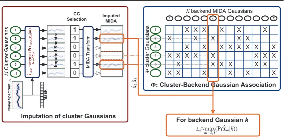
association matrixF(as shown in Figure 2) is incremen-ted by 1. After all training data are processed, the setΩk in Equation (12) is defined from thekth column ofFas those entries that are larger than the product of a prun-ing thresholdθF and the maximum of thekth column. Moreover, ifΩkcontains more thanLmaxelements, only theLmaxlargestF-values are retained. The entries ofF that are not inΩkare subsequently set to zero.
The probability how often CG mis associated with any BGs is formulated by
P(m) =
K
k=1
δmk
M i=1
K k=1
δik
δmk=
1if mk>0
0if mk= 0 (18)
and is used as the prior probability of a CG below.
4.4. Application of MC MDT in the recognizer
Ls m=1
Pmxˆt,u,m,yt,r
> ρ M
i=1
Pixˆt,u,i,yt,r
(19)
where xˆt,u,m is the imputed value from CGm. The CG
are reordered such that
Pmxˆt,u,m,yt,r
≥Pm+ 1xˆt,u,m+1,yt,r
and
Pmxˆt,u,m,yt,r ∼
= p
ˆ
xt,u,m,yt,rm α
P(m)
M i=1
pxˆt,u,i,yt,ri α
P(i) (20)
The exponent a is introduced to compensate for unmodeled correlations among the features and will indirectly control the number of selected BGs. A typical value of a is 0.4, which led to a reasonable trade-off between the number of selected BG and recognition accuracy on the development dataset used in [36]. P(m|ˆxt,u,m,yt,r) denotes the posterior probability of CG mbased on its imputation. In Figure 2, the CGs labeled with “1” in the CG selection table are selected at frame t. Only the imputed clean spectra resulting from the selected CGs are transformed into the MIDA domain and maintained as possible candidates for BG likelihood evaluation.
When calculating the likelihood of a particular BG k, the MC MDT recognizer looks up the kth column of
the CG-BG association table F to find the candidate list. Notice that some of the associated CGs may have been pruned by criterion (19) and are removed from the list. The recognizer calculates the likelihoods of the BG for the candidates of imputed clean speech and selects the maximum as the likelihood of that BG. If the candi-date list is empty, the BG is assigned a likelihood of zero. On average, the number of multiplications involved per BG is reduced to 2LD¯ m, where L¯ is the
average number of CGs associated to a BG and Dm is the dimension of MIDA features. The resulting likeli-hoods of the BGs are used to calculate the state output PDFs, which are then processed by the decoder.
5. Selection of CG
The MC MDT system can be further sped up by apply-ing Gaussian selection on the CGs. ThoughM<<K, the evaluation of a CG is still an order of magnitude more expensive than the evaluation of a BG. Thus, only the likely CGs are selected to impute the candidate clean speech. Existing methods of Gaussian selection can be classified as axis indexing-based methods [37,38] and VQ-based methods [39,40]. The former quickly locates the likely regions based on the observation, then selects the Gaussians in the likely regions [38] or removes the Gaussians in the unlikely regions [37]. But in MDT sys-tems, it is not straightforward to determine which regions in the feature space are likely, because some of
X X X X
X X
X X X
X
X X X X
X X X X X
X X X X
X X X
X X X X
X X X X X
X X X
1 k K
1
2
3
4
5
...
Φ:Cluster-Backend Gaussian Association
Kbackend MIDA Gaussians
M
cluster
Gaussians
X
M
Cluster
Gaussians
Imputation of cluster Gaussians
xt,u,m
=
argmaxP(
xt,u,m
,
yt,r
|
m
)
xt,u,m
≤yt,u 1
2
3
4
5
...
Imputed MIDA
Imputed
Spectra
Noisy
Spectrum:
yt
0
0
0
1
1
0
0
1
1
Mask
1 1 0 0 1 0
MIDA
Transform
For backend Gaussiank Lk≈mmax(P=2,5 (xm|k)) CG
Selection
^
x2,
x5
^
^
^
the components of the observation are missing. On the contrary, VQ-based methods suit the MC MDT system well. Cluster-of-Cluster Gaussians (CCG) in the PRO-SPECT domain are now established. The MC MDT recognizer will select the CGs based on the likelihoods resulting from the imputation of CCGs, i.e., an addi-tional layer of Gaussian selection is provided. Conse-quently, it reduces the number of CG CLSQ problems to be solved. Clustering of the CGs is a prerequisite for the VQ-based Gaussian selection. In this study, we apply the soft K-Means algorithm to generate the CCGs. Since the CCGs and the CGs are expressed in the same domain (PROSPECT features in our example), a model-based approach is feasible and preferred here.
5.1. SoftK-means clustering
The following pseudo code summarizes the steps to obtain the CCGs. A single cluster is first calculated using all the CGs. The number of CCGs then grows incrementally from 1 toNto avoid suboptimal cluster-ing as much as possible.
1. Set the number of CGnto 1 and compute a sin-gle CCG from all CGs.
2. Whilen<N
2a. Find CCG ˆj with the maximum mean WSKLD
2b. Split CCG ˆj into two and increment n 2c. For iterationτfrom 1 toT
2c-1. For CCGi,ifrom 1 ton 2c-1-1. For CGm,mfrom 1 toM
Calculate the weight by which CGmupdates CCGi,ĝ(i, m)
2c-1-2. Givenĝ(i, m), updateμi, Σiiteratively The distance metric between Gaussians and the com-putation of the CCGs from its member CGs are two crucial components for every step listed in the above pseudo code. The distance metric is Weighted Kullback-Leibler Divergence (WSKLD) in step 2a and is explained in Section 5.2. The parameter estimation algorithms in steps 1, 2c-1-1, and 2-c-1-2 are described in Section 5.3. Step 2b is described in Section 5.4.
5.2. Distance metric between PROSPECT Gaussians
The symmetric Kullback-Leibler Divergence (SKLD) is commonly used to measure the distance between CCG nand CGm:
SKLD(n,m) =1
2trace
(n−1+m−1)(µn−µm)(µn−µm)+n−1m+nm−1−2I
The application of SKLD to (14) requires some care: the stream exponent b in the likelihood model for
PROSPECT features makes it an improper distribution, requiring renormalization such that it integrates to unity. Second, it was found that SKLD overweighs dif-ferences in the projection part of the PROSPECT Gaus-sians. Therefore, in [41], further simplifications were proposed and experimentally verified leading to the WSKLD as a clustering metric for multi-stream features:
WSKLD(n,m) =
Nstrm
j=1
βjSKLDj(n,m)
where bj is the exponent of stream j, SKLDj is the symmetric KLD computed on the features of stream j only and Nstrmis the total number of streams. In this study, Nstrmis 6 because the PROSPECT features con-tain static, velocity and acceleration stream of both cepstral and projection parts.
5.3. Parameter estimation of CCGs
Following the K-Means algorithm in [42], the cost func-tion to be minimized for clustering is
QK−Means= M
m=1
N
n=1
g(n,m)WSKLD(n,m) +γ
N
n=1
g(n,m) log 1 g(n,m)
(21)
wheregcontrols the stiffness of the clustering andg(n, m) are unknown clustering weights. The parameters to be updated iteratively are
[µˆn,ˆn,ˆg(n,m)] = arg min
µn,n N
n=1 g(n,m)=1
(QK−Means)
In each iteration, the first step is to obtain the optimal weight by which CGmaffects CCGnas
ˆ
g(n,m) = exp(−WSKLD(n,m)/γ)
N i=1
exp(−WSKLD(i,m)/γ)
The second step is to find the optimal values of mean and covariance of each CG given the weights. The esti-mation of means and covariance matrices of the CCGs is based on the approach in [43], where a method for finding the centroid of a set of Gaussians is derived. The centroid is the CCG that minimizes the sum of the WSKLD to all CGs. Here, we extend the results of [43] by modifying the cost function to (21). The mean of a CCG is thereby estimated as
ˆ
µn=
M
m=1 ˆ g(n,m)(−1
m +−n1)
−1M
m=1 ˆ g(n,m)(−1
m +−n1)µm
(22)
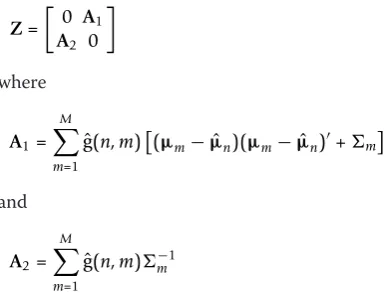
Z=
0 A1
A2 0
where
A1= M
m=1 ˆ
g(n,m)(µm− ˆµn)(µm− ˆµn)+m
and
A2= M
m=1 ˆ
g(n,m)−m1
By construction,ZhasDPpositive and DP symmetri-cally negative eigenvalues, whereDP is the dimension of PROSPECT features. A 2DP-by-DP matrix V is con-structed whose columns are the DPeigenvectors corre-sponding to the positive eigenvalues.V is partitioned in its upper halveUand lower halveW:
V=
U W
ˆ
n=UW−1 (23)
Like in [43], ˆn is constrained to be diagonal during clustering. It can be seen from Equations (22) and (23) that the procedure of estimating the CCGs given the weightsĝ(n,m) is iterative. The calculation of the mean depends on the previously calculated covariance and vice versa. The exit criterion is the convergence of the cost function defined in Equation (21).
In step 1 of the pseudo code from Section 5.1, a single CCG is initialized by averaging the means and covar-iance matrices of the entire set of CGs. The parameters of the single CCG are then updated using Equations (22) and (23) for several iterations. Splitting a CCG and re-estimation of all CCGs are carried out iteratively till NCCGs are obtained, as explained below.
5.4. Splitting a CCG
In each iteration, the CCG with the maximum within-cluster mean WSKLD is found
ˆj= arg max
j=1...n M m=1
ˆ
g(j,m)WSKLD(j,m)
M m=1
ˆ
g(j,m)
Principal component analysis is applied on the covar-iance matrix ˆj to find the first principal eigenvectore1 and eigenvalue,l1. If the number of CCGs in the current
iteration isn, CCG ˆj is split into two Gaussians with the means and covariance matrices:
µn+1←µˆj+ξ
λ1e1
µˆj←µˆj−ξ
λ1e1
n+1=j=ˆj
whereξis the disturbing rate. The WSKLDs of all the M CGs to the newly created CCGs is then calculated. Each weight gˆ(ˆj,m) is also split into two according to the WSKLDs:
ˆ
g(n+ 1,m)← exp(−WSKLD(n+ 1,m)/γ)g(ˆˆj,m) exp(−WSKLD(n+ 1,m)/γ) + exp(−WSKLD(ˆj,m)/γ)
ˆ
g(ˆj,m)← ˆg(jˆ,m)− ˆg(n+ 1,m)
The parameters of CCG ˆj and CCG n + 1 are then re-estimated using Equations (22) and (23) with fixed number (e.g., 3) of iterations. The means and covariance matrices of CCG 1 to n+ 1 are subsequently updated until convergence of the global cost function (21).
Finally, whennreaches N, anNby MCCG-CG table of exponentiated negative WSKLD is calculated. This table plays the same role as the association table in Sec-tion 4.3. The same schemes as in SecSec-tion 4.3 are used to truncate the table. Also, the same schemes as in Sec-tion 4.4 are used to select likely CGs, thus avoiding sol-ving CLSQ problems whose solutions are unlikely to survive pruning criterion (19).
6. Experiments
6.1. Data and models 6.1.1. AURORA-4
Speech recognition experiments were conducted on the AURORA-4 database [44], a large vocabulary task that is derived from the WSJ0 Wall Street Journal 5k-word dictation corpus. A bigram language model for a 5k-word closed vocabulary is provided by Lincoln Laboratory.
For training, only clean-condition data sampled at 16 kHz were used, consisting of 7,138 utterances from 83 speakers, which amounts to 14 h of speech data. All recordings are made with the close talking microphone and no noise is added.
The test database is composed of 330 read sentences (5,353 words) from 8 different speakers. Fourteen differ-ent versions of this set are created. The first dataset is clean and is recorded with the same close-talk micro-phone as used while recording the training data. It is artificially corrupted by adding six types of noise to establish datasets 2-7: car (set 2), babble (set 3), restau-rant (set 4), street (set 5), airport (set 6), and train (set 7). Set 8 is recorded with far-talk microphones. Test
sets 9-14 are created by artificially adding the same six types of noise as used for generating sets 2-7. Each test set contains 330 utterances and has an SNR that ranges from 5 to 15 dB.
6.1.2. Training backend acoustic model
The design of the front-end as well as the backend acoustic model is based on prior study [23,33,37] which obtained competitive accuracies on clean speech and good robustness in an MDT configuration.
The signal power spectrum is calculated with a 32-ms Hamming window and a 10-ms window shift and is integrated using a 22-channel MEL-scaled triangular fil-ter bank with lowest frequency cenfil-tered at 140 Hz to increase the robustness to low-frequency noises. Since all frequencies above 7 kHz of the AURORA-4 data are filtered out, the last band is centered at 5800 Hz. The 22 log-spectral coefficients are mean-normalized and the first- and second-order time derivatives are appended to result in 66-dimensional spectral features.
To train the backend acoustic model, the normalized spectral features are transformed into 39-dimensional MIDA features, which are improved LDA features
Table 2 WER of the MC MDT experiments on test set 1-7 (Close-talking microphone)
WER (%)
1. Clean 2. Car 3. Babble 4. Restau. 5. Street 6. Airport 7. Train Average
1. No MDT 6.82 12.98 32.62 40.95 38.50 32.51 38.37 28.96 ± 0.5
2. BE PROSPECT MDT 6.33 10.89 20.14 28.38 25.42 20.57 25.14 19.55 ± 0.4
3. GB GD MC MDT 6.28 10.95 20.08 29.76 24.98 20.18 25.28 19.64 ± 0.4
4. GB MAP MC MDT 6.00 10.31 20.90 29.12 24.86 19.73 25.89 19.55 ± 0.4
5. GB GD MC MDT + CGS 6.16 10.93 20.36 29.48 25.72 19.91 25.13 19.53 ± 0.4
6. GD CLBR 6.18 11.96 22.90 31.22 26.60 21.74 29.03 21.38 ± 0.4
7. MAP CLBR 6.28 11.81 21.69 31.44 27.63 21.74 28.51 21.30 ± 0.4
8. SB MC MDT 6.67 11.25 20.25 28.90 24.49 19.67 25.20 19.49 ± 0.4
9. Spectral MC MDT 6.41 10.46 21.63 29.68 25.89 20.66 25.85 20.08 ± 0.4
10. Cepstral MC MDT 6.44 11.04 19.90 29.46 25.61 19.86 26.53 19.83 ± 0.4
GB, Gaussian-based; SB, State-based; CGS, CG selection; CLBR, cluster-based reconstruction; BE, Backend.
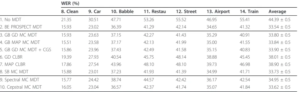
Table 3 WER of the MC MDT experiments on test set 8-14 (Far-talking microphone)
WER (%)
8. Clean 9. Car 10. Babble 11. Restau 12. Street 13. Airport 14. Train Average
1. No MDT 21.35 30.51 47.71 53.26 55.52 46.95 55.41 44.39 ± 0.5
2. BE PROSPECT MDT 15.93 23.02 36.39 41.29 42.14 34.65 41.32 33.54 ± 0.5
3. GB GD MC MDT 15.93 23.63 37.15 42.27 41.43 35.29 40.91 33.80 ± 0.5
4. GB MAP MC MDT 15.51 23.58 37.17 42.13 41.99 35.00 41.55 33.84 ± 0.5
5. GB GD MC MDT + CGS 15.86 23.96 37.43 42.49 41.58 35.15 40.83 33.90 ± 0.5
6. GD CLBR 19.39 27.93 40.54 45.75 48.14 38.88 45.45 38.01 ± 0.5
7. MAP CLBR 17.86 27.54 43.96 48.10 48.10 39.73 46.98 38.90 ± 0.5
8. SB MC MDT 15.88 23.01 37.23 41.93 41.39 34.99 41.71 33.73 ± 0.5
9. Spectral MC MDT 15.77 24.42 38.74 44.57 42.42 36.17 42.54 34.95 ± 0.5
10. Cepstral MC MDT 16.05 23.04 36.57 42.37 41.74 35.07 41.84 33.62 ± 0.5
leading to decorrelation and diagonalization of the mix-ture components [34]. It has only half the dimension of PROSPECT features (see Section 6.1.3), hence leading to a significant effort reduction in the likelihood calcula-tion of the BGs and showing better accuracy than MFCC.
The acoustic model uses cross-word and context-dependent triphones. The HMM for each triphone con-tains three states. A PDT defines 4091 tied states, or senones, which in their turn share 21,037 BGs. The out-put probability of each state is a mixture of 190 BGs on average and each Gaussian is shared among 45 different tied states.
6.1.3. Training CGs and CCGs
The compact acoustic model containing the CGs is trained with the same training data by following the training procedure outlined in Section 4.2. Here, the state-level segmentation of the training data is obtained by forced alignment using the backend MIDA model of
Section 6.1.2. The normalized static log-spectral features and the dynamic features are transformed into PRO-SPECT features withDc= 4, i.e., for each stream in the features, four cepstral coefficients are kept, andD= 22 projection coefficients are appended. Consequently, the PROSPECT features including delta’s have 78 dimen-sions. An earlier experiment on AURORA-4 showed that MC MDT with 500 to 900 CGs yields a reasonable trade-off between recognition time and accuracy. Therefore, we use 500 CGs in the following experiments. The associa-tion tableFis built on the same training data. The maxi-mum number of CGs associated with a particular BG, Lmax, is 5. An earlier experiment on the Flemish Speecon and SpeechDat Car data [36] showed that increasingLmax beyond 5 only leads to more computation without increasing the recognition accuracy. The average number of CGs associated with a particular BG,L¯, is 3.6.
Fifty CCGs are obtained by clustering the 500 CGs using the procedure from Section 5. The maximum
Table 4 Average CPU time breakdown over test set 2-7
CPU time (ms/frame) BG calculated (%)
Mask estimation BG Calculation CG Evaluation Beam Search Total
1. No MDT 0.0 3.5 0.2a 24.4 28.1 27
2. BE PROSPECT MDT 1.1 133.5 0.0 18.5 153.1 100
3. GB GD MC MDT 1.1 2.8 4.3 20.0 28.2 11
4. GB MAP MC MDT 1.1 3.3 7.6 22.2 34.2 13
5. GB GD MC MDT+CGS 1.1 2.4 1.2 19.1 23.8 9
6. GD CLBR 1.1 1.3 4.3 19.3 26.0 11
7. MAP CLBR 1.1 1.2 10.6b 18.5 31.4 9
8. SB MC MDT 1.1 30.2 4.6 20.1 56.0 11
9. Spectral MC MDT 1.1 10.4 0.5 23.7 35.7 38
10.Cepstral MC MDT 1.1 2.8 7.0 19.0 29.9 10.5
a
In the case of No MDT, the time for CG evaluation is replaced by FRoG.b
In cluster-based reconstruction with MAP, the time of CG evaluation includes the calculation of the likelihood for 500 PROSPECT CGs, which is equivalent to evaluation of 1000 MIDA Gaussians.
GB, Gaussian-based; SB, State-based; CGS, CG selection; CLBR, Cluster-based reconstruction; BE, Backend.
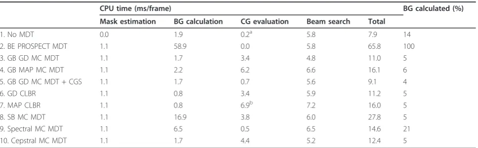
Table 5 CPU time breakdown for the clean condition (test set 1)
CPU time (ms/frame) BG calculated (%)
Mask estimation BG calculation CG evaluation Beam search Total
1. No MDT 0.0 1.9 0.2a 5.8 7.9 14
2. BE PROSPECT MDT 1.1 58.9 0.0 5.8 65.8 100
3. GB GD MC MDT 1.1 1.7 3.4 4.8 11.0 5
4. GB MAP MC MDT 1.1 2.2 6.2 6.6 16.1 6
5. GB GD MC MDT + CGS 1.1 1.7 0.7 5.6 9.1 4
6. GD CLBR 1.1 0.8 3.4 5.9 11.2 5
7. MAP CLBR 1.1 0.8 6.9b 7.2 16.0 5
8. SB MC MDT 1.1 16.9 3.8 6.0 27.8 5
9. Spectral MC MDT 1.1 6.5 0.5 6.5 14.6 21
10. Cepstral MC MDT 1.1 1.7 4.4 5.2 12.4 5
a
In the case of No MDT, the time for CG evaluation is replaced by FRoG.b
In cluster-based reconstruction with MAP, the time of CG evaluation include the calculation of likelihood for 500 PROSPECT CGs, which is equivalent to evaluation of 1000 MIDA Gaussians.
number of CCGs associated with a CG is 5 and the average number is 3.6. In previous experiments on Gaussian clustering, we have found a gof 0.3 in Equa-tion (21) to be a good choice, which we have maintained in these experiments.
6.1.4. Training spectral CGs for the cluster-based reconstruction with MAP
In order to accomplish the experiments of the MAP cluster-based reconstruction for comparison, a mixture of 500 Gaussians with full covariance is trained as well on the spectral data using EM on the same segmenta-tion. As proposed in [24], the initial iterations use a diagonal covariance model that serves to make the pos-terior probability calculation (6) feasible. Only in the last EM-iteration, the full covariance matrices are esti-mated for application in Equation (5).
6.1.5. Training backend PROSPECT model
In order to show the speed improvement of MC MDT over a full MDT system [45], i.e., where the CLSQ pro-blem (11) is solved per Gaussian with GD, an acoustic model with Gaussians estimated on PROSPECT features is required. The model has 21,037 PROSPECT Gaus-sians which are obtained by Single Pass Retraining (SPR) [46] of the acoustic model with MIDA features. The inputs of the SPR are the MIDA features, PRO-SPECT features, and the MIDA model described above. The MIDA model is used to compute the posterior probabilities of every Gaussian over the training data, which are subsequently combined with the PROSPECT feature observations to estimate their GMM weights, means and diagonal covariance matrices.
6.2. Recognizer
6.2.1. Handling convolutional noise
Besides additive noise, the MDT recognizer also handles convolutional noise by the channel compensation tech-nique described in [23], which maximizes the likelihood of the recognized speech on the backend model. To make the implementation tractable, only the contribu-tion of the single Gaussian that gives the largest contri-bution to the state likelihood (the dominating BG) is taken into account. However, unlike in [23], the current approach computes only approximate solution for BGs which is expressed in a different feature domain. There-fore, each dominating BG is replaced by the PROSPECT CG with the largestF-value so the maximum likelihood channel estimation of [23] can be readily applied. The channel estimate is subtracted from the observed log-spectra and hence the CCG, CG, and BG models are all compensated for convolutional distortions.
6.2.2. Mask estimation
The missing data detector used is the method described in [23] which integrates harmonicity and SNR with a speech model based on vector quantization. At each
frame, the best match between a harmonic decomposi-tion of noisy speech and a codebook describing the har-monic decomposition of clean speech is found. VQ mask estimation requires a speech and silence codebook which are trained with a randomly selected subset of the clean training data in Section 6.1.1. The codebook contains 520 codewords which are updated using the channel estimation of Section 6.2.1 during recognition.
6.2.3. Test configuration
The decoding consists of a time-synchronous beam search algorithm as described in [47]. The recognizer was launched on a PC installed with Dual Core AMD Opteron 280 2.4 GHz processors with a cache size of 1 MB. Only one processor core is activated. The MDT imputation is only applied to the static stream, while the first- and second-order time derivatives are uncompen-sated. The Word Error Rates (WER) are calculated for all the experiments. Meanwhile, the CPU time is mea-sured. Tables 2 and 3 list the WERs of the experiments over the 14 types of environmental noises. Tables 4 and 5 contain the timing measurements for the BG and CG evaluation, for beam search as well as the end-to-end timing information (column“TOTAL”) of the recogni-zer under noisy and clean condition, respectively. The timing measurements are achieved by starting and stop-ping (precise) timers frame-synchronously at the entry and exit of each of the different processing steps: front-end processing, CG imputation, candidate evaluation for all BGs, and beam search. The total time is then obtained by dividing the accumulated timings by the number of processed frames over several utterances.
6.3. Baselines
6.3.1. Recognition without MDT
this non-MDT system produces higher WER than the MDT systems under the clean condition (test set 1), as shown in Table 2. This is mainly due to the non-MDT system using spectral mean normalization to reduce the channel effects, while the MDT systems use the more sophisticated MLE-based channel update as described in Section 6.2.1.
6.3.2. Backend PROSPECT imputation
This setup is the most refined previously published ver-sion of our MDT system [23] and serves as a baseline in term of recognition accuracy such that we can measure the accuracy cost of the proposed speed improvements. Two iterations of GD are found to be enough for the convergence in terms of recognition accuracy, hence are applied for all the 21,037 PROSPECT Gaussians. This system runs at 15 times real time in noisy condition and 6.6 times real time in clean condition as shown in row 2 of Tables 4 and 5, respectively. However, the accuracy benefits of MDT can be clearly seen in contrast to the non-MDT system in Tables 2 and 3.
6.4. MC MDT
6.4.1. Gaussian-based MC MDT with GD
The Gaussian-based MC MDT system is an instance of the concepts outlined in Section 4. Two iterations of GD are applied for all the 500 CGs. The posterior probabil-ity-based BG selection described in Section 4.4 is applied.
awas tuned with an isolated word-recognition experi-ment of MC-MDT on the Speecon and the SpeechDat Car databases used in [36], which we hence regard as development data for this article. The tuning experiment shows that a good trade-off between accuracy and BG evaluation effort is obtained ata= 0.4, but that it does not critically affect the recognition accuracy.
Compared to the backend PROSPECT MDT system, i.e., row 2 versus row 3 in Tables 2, 3, 4, and 5, the Gaussian-based MC MDT yields a comparable WER, while it uses less than 20% of the CPU time over the entire test set.
It is remarkable that the Gaussian-based MC MDT works as fast as the non-MDT recognizer with the same backend acoustic model under noisy conditions (row 1 versus row 3 of Table 4). The MC MDT spends time in evaluating CGs, but its decoding time is reduced by 4 ms per frame. Faster decoding on corrupted data is actually a common benefit from MDT imputation as shown in Table 4. In non-MDT systems, the mismatch between data and model results in a lower likelihood for the ground truth hypothesis and also causes many hypotheses to yield a similar score, so pruning is not effective and the decoder slows down. In the MDT sys-tem, noise addition also slows the recognizer down, but through a different mechanism. Thanks to the imputa-tion process in MDT systems, the likelihood of the ground truth hypothesis will not deteriorate. The
likelihood of alternative hypotheses will also increase, but because they do not fit the data well, their imputa-tion benefit is not that strong. Apparently, a significant likelihood gap is maintained among the hypothesis, causing pruning in MDT systems to be more effective than in non-MDT systems. The effort spent in evaluat-ing CGs is recovered in the search.
The increase in the likelihood of alternative hypoth-eses in the MDT system under noisy conditions also causes the MC MDT system with GD to run about 2.5 times slower than under clean conditions (row 3 of Table 4 versus row 3 of Table 5). As the data get noi-sier, the imputation becomes less constrained, since the number of unreliable components increases and the bounds outlined in Section 2.1 become less strict. Hence, the dynamic range of the BG likelihoods will decrease, such that the hypothesis likelihoods will show smaller differences, causing pruning to be less effective. Additionally, the system is slowed down with increasing noise levels because more spectro-temporal regions are labeled as unreliable and the complexity of imputation for CGs and CCGs increases.
Some common advantages of MDT are revealed by the results shown in Tables 2 and 3. All the experiments with MDT produce lower WERs than the non-MDT system over the corresponding noise types, as well as in the clean condition. Especially for the non-stationary noise types, namely, set 3-7 and 10-14, the benefit from MDT is more significant.
Though MDT systems show an advantage in both the close-talk and the far-talk test sets, the performance is greatly degraded in the latter condition, because the channel compensation technique of Section 6.2.1 is restricted to the estimation of a log-spectral offset vec-tor, which can only compensate for convolutional effects with a short impulse response. However, the fact that the backend PROSPECT MDT and the MC MDT sys-tem perform equally on this test set confirms that the modification to estimate the channel on CGs rather than on BGs (see Section 6.2.1) works.
6.4.2. Gaussian-based MC MDT with MAP
6.4.3. Gaussian-based MC MDT with CG selection
The CG selection introduced in Section 5 is added to the Gaussian-based MC MDT system in Section 6.4.1. In addition to the 50 PROSPECT imputation operations for the CCGs, about 106 PROSPECT imputation opera-tions for the CGs are observed per frame of 10 ms. Therefore, the number of CLSQ problems solved is less than one-third of that of MC MDT without CG selec-tion. Two iterations of GD are applied on the imputa-tion of CCGs. The implementaimputa-tion of Gaussian-based MC MDT plus CG selection does not harm the recogni-tion accuracy but consumes less CPU time in compari-son with the Gaussian-based MC MDT system (compare row 3 with 5 in Tables 2, 3, 4, and 5).
6.4.4. State-based MC MDT
The imputed values of the Gaussian-based MC MDT described in Section 6.4.1 can also be used to perform a state-based MC MDT, where the imputation for state s is the linear combination of the imputed values from the BGs included in the GMM of that state.
ˆ
xt,u,s =
k∈GBG(s)
Pkxˆt,u,k,yt,r,s
ˆ
xt,u,k (24)
whereGBG(s) represents all the Gaussians belonging to the GMM of states, and
Pkxˆt,u,k,yt,r,s
= p
ˆ
xt,u,k,yt,rk
P(k|s)
j∈GBG(s)
pxˆt,u,j,yt,rj
P(j|s) (25)
The BG selection from Section 4.4 is also activated for this experiment, so only the selected BGs are actually involved in the imputation formulae. Each BG is shared among about 45 states and is therefore evaluated at multiple imputed spectra from its owner states. Hence, for this state-based MC MDT experiment, every selected BG is evaluated at 45 states-based imputed spectra as
ˆ
xt,u,s in Equation (24). The MC-based likelihood
estima-tion of each BG is still performed at 3.6 (average num-ber of CGs assigned to each BG) candidate spectra. These likelihood evaluations lead to a computationally expensive implementation. State-based MC MDT yields WERs fairly close to those obtained in other MC MDT experiments, but with a significantly higher computa-tional cost, as shown in the 8th rows in Tables 2, 3, 4, and 5.
6.5. Cluster-based reconstruction
6.5.1. Cluster-based reconstruction with MAP
This experiment is an instance of the concept formu-lated by Equations (4), (5), and (6). Each of the 500 full-covariance spectral CGs is used to impute clean speech with six iterations of the MAP imputation. The
corresponding diagonal-covariance CGs are used to cal-culate the definite integrals in Equation (6). To compen-sate for unmodeled correlations, the integrals are exponentiated with 0.3, a value that is tuned on the test set for best accuracy. The global clean spectrum is then reconstructed using Equation (4). Since the likelihoods of the 500 CGs are already calculated, they are used to select BGs as explained in Section 4.4. Despite the test set optimization, the cluster-based reconstruction with MAP imputation is still less robust than the MC MDT systems when comparing row 7 with rows 3, 4, 5, and 8 in Tables 2 and 3. The use of a more accurate speech model provided by the BGs seems to pay off.
6.5.2. Cluster-based reconstruction with GD
This system approximates the previous one by combin-ing the imputed spectra obtained from the PROSPECT CGs like in Equation (4), but takes a different approach to compute the posterior probabilities of the CGs. These posteriors are calculated by renormalizing the likelihoods of the imputed clean spectra. The likelihoods also serve for BG selection as explained in Section 4.4. To compensate for unmodeled correlations, the likeli-hoods are exponentiated with 0.3, a value that is also tuned on the test set for best accuracy. We did not observe a significant accuracy gain beyond the 500 PRO-SPECT CGs used to report the results in the tables. The approximations outlined above do not harm the robust-ness as shown by a comparison between the rows 6 and 7 of Tables 2 and 3, but this implementation is faster because GD imputation is more efficient than MAP and the computation of the posterior probabilities are sim-plified. Again, despite the test set optimization applied for this cluster-based reconstruction method, MC MDT outperforms it as well.
6.6. Imputation using log-spectral and cepstral CGs
Using a PROSPECT feature representation for the CGs in MC MDT experiments is an implementation choice motivated by speed considerations (see Section 4.1). The CGs can also be trained with other features, e.g., cepstra or log-spectra. To accomplish the comparison of the MC MDT system using CGs in these domains, same number, namely 500 of cepstral CGs and log-spectral CGs are trained using the same data-driven approach as described in Section 6.1.3.
6.6.1. Cepstral imputation