THIS THING CALL CONTROL!
By
Papa Mohd Sulhi bin Azman
2 June 2011
My beloved children,
1. I have noticed that some of you are still probably lost when it comes to control system. And in class, I have also noticed that some of you are with either Alice or Alex in Wonderland. But that is still okay – I just do not want you to turn greener than the goblin, when it comes to control system. The subject is pretty tough and the mathematical treatment of this subject is quite advanced. Therefore, in the event that you do not understand a thing or two, please do not hesitate to come and see me. I’d be more than happy to entertain your questions. Anyway, to make life easier, allow me to highlight few important and salient points about control system so as to further enlighten you on this subject.
2. My child, as you know, this subject is called ‘control systems’, meaning to say that in this subject, we are going to deal with the control of any system: be it mechanical or electrical system. The chief aim of control is to ensure that our system is stable. If it is stable, then the system will work properly and if it is not, then the system will go into the state of chaos; hence the need to control it.
3. In controlling the system, we first need to analyze the performance of the system. But, before we analyze a system, we need to know the model of the system, and in engineering, a model is always referred to a ‘mathematical model’. There are three ways of modeling a system, and it includes but not limited to (a) modeling equation (ME); (b) transfer function and (c) state space. 4. Now, allow me to speak on the topic of ‘modeling equation’. A ME is an equation that describes
the system. Usually, the ME is the differential equation. And in this course, we tend to deal with either first or second order differential equation. To derive a modeling equation, we need to begin with basic and fundamental laws of physics – the conservation law. In layman terms, the conservation law simply states that energy is neither created nor lost; it is simply transferred or conserved. Mathematically, we say that if the system is conserved, then the sum of energy is equal to zero or in other words, the input energy equals to the output energy.
5. Let us consider the mechanical system. The conservation law of mechanical system says that the sum of force equals to zero. However, I prefer to say that the input force equals to the output force. It makes sense, doesn’t it? Whatever comes in must comes out. Hence:
6. Similarly, in electrical system, we also conserve two parameters: current and voltage. Therefore, in any electrical system:
iin=iout and vin=vout
7. Let’s move on. Now, once we have obtained the ME, we can then represent the equation in either transfer function or in state-space. A transfer function is always represented in frequency domain. Sometimes, the frequency domain is simply known as s-domain. Don’t even ask why they use the letter ‘s’. Please spare me your ‘smart’ questions; at least for now ☺ A transfer function is simply known as the ratio between the output function to the input function. Mathematically:
1
1
( )
Output Transfer Function
Input ( )
n i i n i i s z s p = = + = = +
Π
Π
8. Now, how do we obtain a transfer function? It is very simple. All we need to do is to take the forward Laplace transform of the ME and always-always-always assume zero initial conditions. In doing so, please bear in mind that:
[ ]
[ ]
[ ]
2( ) ( ) ( ) ( ) ( ) ( ) ( ) ( ) n n n
L x t X s
L x t sX s
L x t s X s
d x t
L s X s
dt = = = = ɺ ɺɺ
9. In a transfer function, we have two other important parameters that is important when it comes to the concept of stability: the zero and the pole. A zero is a number that makes the numerator equals to zero, and likewise, a pole is also a number that makes the denominator equals to zero. 10. You can sketch the location of the pole and zero in s-plane1 if you wanted to analyze the stability
of the system. But before you do so, you must take note that a zero is drawn as a circle in s-plane and a pole is drawn as a cross. And in your s-plane, the horizontal axis is the ‘real’ axis while the vertical axis is the ‘imaginary’ axis. Sometimes, the vertical axis is simple known as the jω-axis.
11. If either the pole or the zero is located in the right-half of the plane (RHP), then your system is simply unstable. Otherwise, if your pole or zero is located in the left-half of the plane (LHP) then your system is a stable system. Now, what happens if your pole is located in the zero-line? In this case, we say that your system is so-so stable – of course, the proper term is the marginally stable.
12. A state-space (SS) is simple a matrix representation of your ME. I you want to represent your ME in SS, then what you need to do is that you need to determine the state variables. The number of state variable is simply equal to the higher order of derivatives in ME. Suppose that you have a second-order ME. Then, the number of state variables is two. Mathematically:
( )
n
n n d x t
x
dt =
Now, the state variable is always arranged in this fashion:
1
2
(n 1)dot
n
x x
x x
x x
−
= =
= ɺ ⋮
13. The complete SS equation is shown as follows:
x Ax Bu
y Cx Du
= + = + ɺ
Where A is the system matrix and B is the input matrix. Note that the word matrix and vector is sometimes loosely used interchangeably.
14. Okay, what have I talked so far? I have covered (a) modeling equation, (b) transfer function and (c) state space. Now, let’s look a bit into the stability of the system.
15. The stability of a system can simply be determined by (a) using the final value theorem or (b) looking at the location of the pole(s) or zero(s). As I mentioned earlier, if either your pole(s) or zeros(s) is in the RHP, then your system is immediately an unstable system.
instance, we speak nicely to people, we learn to thank you when we have obtained something and we also say please when we need something. All of these changes evolve with time. Now, we can represent our dynamic behaviour mathematically:
Initial Value Theorem
0
(0) lim ( )
t
f f t
→
=
Final Value Theorem ( ) lim ( )
t
f f t
→∞
∞ =
Now, allow me to deliver a quick sermon about behavioural changes. Change is good. But you must work towards changing into good things. If your behaviour changes to good thing, then we say that your behaviours or attitudes are converging (approaching) to a final value. This is what we call a stable system – settling into some final value. And this final value is what bounds us to be who we are.
You can look at it this way: if you are working towards a long-term goal (final value) as time progresses, then you are a ‘stable’ person. You are bounded, restricted and confined to work towards your goal. In summary:
Stable System Mathematically
speaking
• Converge (approach) towards a certain value.
• The system is bounded. Analogy • Work towards your goal.
In summary • Stable person = works towards attaining your goal and dream
But if your behaviour constantly changes with time, and this change keeps diverging and not approaching any value or goal, then definitely you are not a stable system. Why is that? Because you keep changing here and there and you are not settling to anything or any goal or any value in your life. In summary:
Unstable System Mathematically
speaking
• Diverge towards a certain value.
• The system is unbounded.
Analogy • Being clueless and having no goal in your life. In summary • Unstable person = no finite goal in life
17. And one more thing children of the present and leader of future: to have a stable society, your system must be bounded, confined and restricted with laws, rules and regulations. An unstable and chaos society is neither bounded nor confined to any laws, rules and regulations.
19. Okay, that’s that about stability. Now, let’s look at the response of the system. There are two types of response: the time response and the frequency response. We study the frequency response when we have periodic or sinusoidal inputs. We study the time response if our input function is non-periodic.
20. To obtain a time response from a transfer function, we simply take the inverse Laplace transform of the transfer function. Mathematically:
1
( ) [ ( )]
f t =L− F s
21. In control system, we tend to deal with two case of system: the first order (F1) system and the second order (F2) system. The general F1 system is defined by the following equations:
1 a
F
s a
= +
We take note that the highest power of s is one. And we take the inverse Laplace transform of this function, we see that the response is an exponential function.
22. The general F2 system is defined by the following equations: 2
2 2 2
2
2
n
n n
b F
s as b s s
ω
ζω
ω
= =
+ + + +
We take note that the highest power of s is two. And we take the inverse Laplace transform of this function, we see that the response is not necessarily an exponential function. It can be exponential functions is the denominator can be factorized into linear terms. However, if the denominator of this equation cannot be factorized into linear factors, then the response is sinusoidal; because when we take the inverse Laplace transform, we have to complete the square and then we will have an oscillatory term (the sin term).
23. In F2 system, we have to important parameters: the zeta (
ζ
) and the omega-n (ω
n).ζ
is usually known as the damping ratio whileω
n is commonly referred to as the natural frequency. The higher the value ofζ
, the less oscillatory the response would be.Figure 1 The equation describing this sytem is given as:
0
in out
F F
mx kx
= = ɺɺ+
Now, let us solve this differential equation by using classical method (not Laplace transform). We see that the system’s response is:
(
0)
( ) cos
x t =A
ω
t+φ
Where
ω
0= k m. The value of A andφ
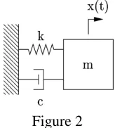
can be determined by using the initial conditions (displacement & velocity). When we plot x t( ), we see that the system will vibrate continuously. This sytem is without a damper.25. What happens when we add a damper? The damper will reduce the vibration of the system. Consider the system in Figure 2:
Figure 2 Let us now model the system by deriving the ME:
0
in out
F F
mx cx kx
=
= ɺɺ+ +ɺ
When we solve the equation by using classical method, we see that the response is:
(
)
( ) tcos
d
x t =Ae−α
ω
t+φ
that the response of the system will decay to some finite value. This can be proved by plotting it in MATLAB (refer to Figure 3):
Figure 3
Therefore, we can conclude that by adding the damper, the vibration will decay or converge to some finite value.
26. Now, for F2 systems, we can analyze the performance by looking at the values of the damping ratio
ζ
. The higher the value ofζ
, the lesser the oscillation. This fact is summarized in Figure 4. We also take note that if the system have no damping ratio, then we say that the system is undamped (durh!). And furthermore, if there is a damping ratio, we can further categorize the system into underdamped, critically damped or overdamped. The following relation, summarized in Table 1, indicates the damping of the system:Table 1
Condition Damping Type
0
ζ
= Undamped0< <
ζ
1 Underdamped1
ζ
= Critically damped1
ζ
> Overdamped27. And now, for stability of F2 system, we can also look at the location of the pole. If the pole is on the RHP, then the system is definitely unstable and the output will be oscillatory. If the pole is on the LHP, then the system is stable, and therefore, it will converge towards a finite value.
Children of God, I end my rants, ramblings and sermons now before I bore you guys to death. Please note that this note is not a substitute of the textbook! It is simply a supplementary note that should complement the textbook that we are using now.
My child, if you are still confused, then I suggest that you put aside this note for a while, get some sleep and then go over it again once you have cleared your mind from the worldly distraction of internet (that includes facebook!) and girlfriends/boyfriends.
As I have also mentioned countless of time, I can be reached via email at [email protected]. I’d be happy to entertain your questions ☺
Adios, amigos!
MOHD SULHI BIN AZMAN Preacher and Advocate Control Systems Engineering June 2nd, 2011 at 3.35am.