Crime, cash, and limited options: Explaining the
prison boom*
William Spelman
University of Texas
Research Summary
An analysis of a state panel of prison populations from 1977 to 2005 shows that the best predictors of prison populations are crime, sentenc-ing policy, prison crowdsentenc-ing, and state spendsentenc-ing. Prison populations grew at roughly the same rate and during the same periods as spending on education, welfare, health and hospitals, highways, parks, and natu-ral resources. Current and lagged values of state spending on prison construction also accounted for a substantial amount of variation in subsequent prison populations. Public opinion, partisan politics, the electoral cycle, and social threats seem to have had little effect on the number of prisoners.
Policy Implications
The availability of publicly acceptable alternatives to incarceration may not be sufficient to reverse course. Federal funding of alternatives—but not prisons—would provide states with the financial incentive to reduce prison populations.
Keywords: prison population, correctional spending, sentencing policy
* The author is grateful to Steven Raphael and Steven Levitt for providing data, to the Policy Research Institute at the University of Texas for its financial support, and to Philip Cook, Michael Murray, and four anonymous reviewers for their valuable suggestions on modeling and analysis. Any remaining errors are the fault of mischievous gremlins. Direct correspondence to William Spelman, LBJ School of Public Affairs, University of Texas at Austin, P.O. Box Y, Austin, TX 78713-8925 (e-mail: [email protected]).
CRIMINOLOGY & Public Policy
Volume 8 Issue 1 Copyright 2009 American Society of Criminology
The United States houses a greater proportion of its citizens in prisons than any other country in the world—more than Russia and China, more than South Africa during apartheid, and maybe even more than North Korea (Walmsley, 2007). The direct costs of incarceration are in excess of $20,000 per prisoner. Many economists think the total social costs, which include legitimate income forgone by prisoners and reduced life prospects for their families, are roughly twice that (for example, Donohue, 2007; Kleykamp, Rosenfield, and Scotti, 2008). Evidence suggests that we have obtained some value for our money. Estimates vary widely, but the margi-nal prison bed seems to prevent somewhere between two and seven crimes, which saves potential victims between $4,000 and $19,000 per year (Levitt, 1996; Spelman, 2005; Western, 2006).
But note the details: If each prison bed reduces costs by no more than $19,000, but costs us $20,000 to $40,000, then do we need this many beds? Clearly not, and it is not (too) difficult to use current estimates of the crime-control effectiveness of prison, the costs of crime to victims and nonvictims, and the costs of prison to show that we overshot the mark sometime in the early 1990s. Enormous cutbacks—reductions of 50% or more in the prison population—are not difficult to justify and would prob-ably save the U.S. public billions of dollars each year.1 Certainly, there is
little economic justification for continuing to build.
1. The elasticity of crime rates with respect to prison rates h is defined as (DC/C) / (DP/P), where C is the number of crimes reported per 1,000 population and P is the number of prisoners per 1,000 population. Then, the number of crimes reduced by put-ting one additional inmate in prison is equal to DC = hC/P. We must adjust for nonreporting by dividing C by the reporting rate; in 2005, this rate was about .57 for violent crimes and about .40 for property crimes nationwide (Catalano, 2006). Miller, Cohen, and Wiersema (1996) show that the average cost of a violent crime to the victim is $13,000, and the average cost of a property crime is $1,200 (both in year 2000 dollars). Thus, the average benefit of one additional prisoner is equal to 13000/.57 hvCv+ 1200/
.40 hp Cp. Donohue and Siegelman (1998) show that the average cost of an additional
prisoner is about $36,000 per year (again in year 2000 dollars). If we define the opti-mum level P* as that prison rate where the benefit-cost ratio is exactly 1.0, then it is not difficult to show that P* = .63 hv Cv + .08 hp Cp. If Levitt’s (1996) estimates of hv = –.38
and hp = –.26 are applied to reported crime and prison rates for 2005 for the 50 states,
we find that the average value of P* = 1.69. In 2005, the prison rate in the average state was 4.35. Thus, the average state should reduce its prison population by 1.69/4.35 – 1 ≈ 58%. Optimal state-by-state reductions range from 4% (in Massachusetts) to 82% (in South Dakota). No state should increase its prison populations. If Western’s (2006) con-siderably lower elasticities are used (hv = –.03, hp = –.07), then the average state should
How did we ever get to this point? Why is the prison population so high? No shortage of explanations is available. Some researchers view the prison boom as a straightforward response to the increase in crime during the 1970s and 1980s (although this seems to conflict with increasing prison populations during the crime decrease of the 1990s). Others view prison expansion as a response to demands of an increasingly conservative electo-rate or as a “wedge” issue that imparts a partisan political advantage to those who champion it. Still others argue that prison expansion is a means of shoring up failing social institutions such as the family and the public schools, an attempt at regaining control in an increasingly chaotic society. It is fairly easy to document how we got to this point. The criminal jus-tice system is in some sense a simple machine, in which the number of prisoners is equal to crime rates, times arrest rates per crime, times incar-ceration rates per arrest, times sentences served. This process makes it possible to break down annual changes in prison admissions into their component parts, and it has produced some clear findings. Prison growth during the 1980s was primarily caused by increases in incarceration rates among convicted offenders (Langan, 1991); later increases were mostly caused by increases in drug arrest rates and sentences served (Blumstein and Beck, 1999; Sabol, Rosich, Kane, Kirk, and Dubin, 2002). Although such findings tell us how prison populations increased, they beg the more important question: Why did incarceration rates and sentences served increase? Why did we become more punitive?
Answering questions like these requires another approach. Most empiri-cal tests of this kind are of the familiar form:
PRISON = a + X + e
where PRISONis some transformation of the incarceration rate, X is a
vec-tor of predicvec-tor variables, and a and are coefficients to be estimated. Table 1 shows the results associated with the three most recent and com-prehensive studies. Some findings are consistent across studies: Prison populations seem to increase with the black population and the percentage of Republicans in the legislature and decrease as more is spent on welfare and education. But the effects of crime rates, public opinion, poverty and unemployment, and even sentencing policy are inconclusive, at best. It is difficult to tease a consistent narrative from these findings.2
Table 1. Predictors of prison populations: Previous findings
Greenberg & West Jacobs & Carmichael Smith (2001) (2001) (2004)
Economy
Unemployment rate .193 .056 .110
Poverty rate — — –.119
Underclass Threat
Pct black .445 .080 .242
Pct Hispanic –.049 .039 —
Income inequality .527 — .055
Pct urban –.018 — —
Institutional Failure
Divorce rate — — .065
Public Opinion
Citizen conservatism index .617 .343 .094
Pct religious fundamentalists .076 .090 —
Partisan Politics
Republican governor* .002 — .011
Pct Republicans in legislature — .055 .408
Electoral Cycle
Gubernatorial election year* — — .081
Presidential election year* — — –.074
Crime
Violent crime rate .316 .357 .285
Property crime rate .151 — .030
Drug arrest rate .170 — —
Prison Crowding & Sentencing Policy
Prison crowding court order* –.005 — —
Pct of population on probation — — –.021
Determinate sentencing law* –.020 –.027 –.029
Habitual offender law* — — .010
Marijuana decriminalized* — — –.021
State Resources
State revenues per capita [–2] .197 — —
Real state spending on welfare –.311 — —
Pct GDP spent on education — — –.316
Region
South* –.030 — —
Earliest year included 1971 1971 1980
Latest year included 1991 1991 1995
NT, total cases controlled for 147 150 784
STATE effects No Yes No
YEAR effects Yes Yes No
autoregressive effects Yes No Yes
Dependent variable PRISON log PRISON PRISON
R2 .866 .905 .980
Part of the problem here is technical. All three of these studies used panel data, but two studies relied on waves 10 years apart, whereas the third used annual data. The studies controlled for state and year effects in different ways. All studies relied on a common base of theory and broke down classes of explanatory variables in similar ways, but each study used a different set of independent variables. All studies used the level of the prison population as the dependent variable (either the number of prison-ers or the logarithm), but this technique is liable to produce spurious results if PRISON and its predictors are trending variables (Granger and
Newbold, 1974). Although all these researchers made defensible choices, it is not hard to see how these choices may have affected the results.
A more interesting possibility stems not from differences among these studies but from what they all had in common: All studies attempted to connect prison populations to the economic, social, and political condi-tions prevailing at the time. For example, they measured the effects of Republican control of the state legislature in 1991 on the prison popula-tion in 1991. But the primary effect of Republican control (and other variables) may not have been immediate. The legislature may have author-ized construction of a new prison, which could take years to complete.3
Even an immediate influx of prisoners will have long-lasting effects if prison populations are slow to shift over time.4
belongs to a sect that believes in a literal translation of the Bible) has a within-state standard deviation of .130. This complicates the interpretation of the coefficients. Jacobs and Carmichael report coefficients of .28 (for republicans) and .09 (for funda-mentalists), but this is misleading because a one-unit change in republicans is 18.222/ .130 = 140 times as likely to happen in the average state as a one-unit change in funda-mentalists. In addition, republicans is expressed in terms of percentages (0 to 100), whereas fundamentalists is expressed in terms of the logarithm of the proportion (0 to 1). The dependent variable also differs across studies. The point is that a large elasticity is not necessarily evidence of a large effect, and a small elasticity is not necessarily evidence of a small effect. In the Results section, an alternative method of analysis is used that measures the importance of each group of variables more directly.
3. In 1998, California estimated a time to completion of 42 months after a site was chosen and acquired (Little Hoover Commission, 1998). In the early 1990s, the Pennsylvania average was 5 years (Gauger and Pulitzer, 1991); in Texas, the estimate was “up to seven years,” which included site identification and acquisition (Texas Crim-inal Justice Policy Council, 1992:14).
4. Suppose Pt = fPt–1 + et, where f measures the extent to which prison
popula-tions from the previous period carry over to the next. Then f is the proportion of a one-time-only jolt in population that will carry on to the next period; f2
will carry on two periods in the future, f3
This fact suggests that, in part at least, previous studies looked in the wrong place for their correlates. Today’s unemployment, partisan political control, and per capita crime rates cannot be expected to be accurate predictors of capital spending and incarceration decisions made 5 years ago. It is also possible that the short-term, dynamic effects of changes in unemployment, politics, and crime are different from the long-term, equi-librium effects. To improve the accuracy of our explanations, we need to consider timing and to separate short-term results from long-term outcomes.
The analysis detailed below considers the same social, economic, and political variables as those examined in previous econometric studies. It includes more independent variables and uses current best practices to define the dependent variable and the model. More important, however, it considers timing in two ways. First, it includes capital spending as an inter-vening variable. As shown below, capital spending decisions are predictable and largely respond as expected to changes in current condi-tions and (arguably) to expectacondi-tions of future prison needs; prison populations, in turn, seem to depend on previous capital decisions. Sec-ond, the analysis includes both dynamic and equilibrium elements, and it shows that these two effects differ, for some variables at least. The result is a remarkably simple explanation for what caused the prison boom of the last 30 years: persistently increasing crime rates, sentencing policies that put more offenders behind bars and kept them there longer, and sufficient state revenues to pay for it all.
Data
Most previous econometric explanations of the prison boom rely on either the national time series (e.g., Beckett, 1997; Jacobs and Helms, 1996) or a cross section of states (Beckett and Western, 2001; Michalowski and Pearson, 1990). The usual concerns about these designs apply: At
less) the design used in the three most recent studies described in Table 1.5
As described in the next section, one of the critical dependent variables is only available beginning in 1977, so this period does not cover the entire increase in nationwide incarceration rates, which began in the early 1970s. But it does cover 80% to 90% of it.6
Dependent Variables
Consistent with previous studies, let us measure the prison population as the jurisdictional population per 1,000 state residents. Thus, PRISON
includes not only prisoners in state facilities (the custody population) but also convicted offenders doing state time in local jails, private correctional facilities, federal prisons, and facilities in other states.
Let us also measure P.CAPITAL, which is state spending on land and
building acquisition and on new construction for the correctional system. These figures were taken from the Annual Survey of Governments con-ducted by the U.S. Bureau of the Census.7 Not all of this spending is on
prisons; for the period 1987–2005, roughly 10% of spending was for nonin-stitutional purposes, mostly office space for administrators as well as
5. Both Greenberg and West (2001) as well as Jacobs and Carmichael (2001) relied on a panel of U.S. states with only three time-series observations separated by 10 years (1970, 1980, and 1990). Jacobs and Carmichael relied on both fixed- and random-effects models, and they show that (for these data) the results are very similar. Smith (2004) examined annual state prison populations for 1980–1995 and reported results of a model relying (more or less) on annual differences, which often accomplishes the same result as a fixed-effects model. A fixed-effects model apparently produced very similar findings (Smith, 2004:932, footnote 5).
6. State prison rates bottomed out in 1972, when the rate of prisoners per 1,000 population was .934. By 2005, the rate had climbed to 4.882 per 1,000, which is an increase of 3.948 prisoners per 1,000 and 1.265 million prisoners. The increase between 1977 and 2005 was 3.603 prisoners per 1,000 population and 1.179 million prisoners. Thus, the 1977 to 2005 period accounts for 92% of the total rate increase, and 93% of the total prisoner increase. Results presented later suggest that capital decisions pre-cede prison population increases by 3 to 5 years; nevertheless, the 1982–2005 period accounts for 80% of the rate increase and 84% of the prisoner increase.
probation and parole officers. Nevertheless, no breakdown is available for the 1977–1986 period, and 10% is sufficiently small that we can safely ignore it.8 As usual, we adjust for inflation by using the gross domestic
product (GDP) price deflator.9
Previous research has shown that the prison population is nonstationary; that is, it changes slowly over time, and the best predictor of prison in any given year is the value of prison for the previous year.10 The problem here
is that any other variable that drifts up or down in the same way may seems to be correlated with prisons, even though these two variables are not related. This result is especially likely for variables such as GDP or state spending that, like PRISON, trend over time.
This approach has implications for both the conduct of the research and our interpretation of the findings. From a technical viewpoint, consistent results can be obtained in two ways. One is cointegration: We may find that a long-run equilibrium exists between prison and one or more inde-pendent variables, such that the deviation between the expected equilibrium value of prisoners and the true value is stationary. For exam-ple, we might find that states tend to spend a fixed proportion of GDP on prisons. That is,
Pt = bGDPt + et (1)
where b represents the proportion of GDP. Thus, prison rates and GDP each wander up and down in small increments over time; neither is statio-nary. If the residuals are also nonstationary, then the relationship between prisons and GDP may very well be spurious and caused only by chance. If, however, the residuals are stationary, then prison rates track GDP over time such that the deviation between the two never can be too large. In fact, it can be shown to be self-correcting; large deviations tend to be fol-lowed by smaller ones, as prison rates shift back into place (Engle and
8. An attempt was made to use the pattern of institutional and noninstitutional spending for the 1987–2005 period to predict the proportion of institutional spending for the 1977–1986 period. The best model relied on state fixed effects and a folded log of time. Although statistically significant, the predictions were not particularly accurate (R2
= .423, F(50,899) = 13.157). More to the point, the resulting variable was not as effective a predictor of subsequent prison capacity and population as was total correc-tional capital spending.
9. The more familiar consumer and producer price indices are highly correlated with the GDP price deflator, but these indices focus on consumer items and raw indus-trial materials rather than on construction costs. In practice, experimentation showed that the choice of deflator has no important effect on the results.
10. More technically, PRISONt = Sk bk PRISONt-k, and Skbk≈ 1.0. In the long run, PRISON cannot be exactly unit root. Because we generally define it as a proportion of
Granger, 1987). In this case, we could be sure that Equation 1 measures a true long-run equilibrium relationship and not a spurious one. If we can-not find evidence of cointegration, then we are on shaky ground unless we define the dependent variable, not as the number of prisoners in a given year, but as the change (or percentage change) in prisoners over the previ-ous year. Relying on levels risks spuriprevi-ous results.
Independent Variables
Previous explanations for the prison boom can be roughly divided into five types: social threat, politics, crime control, crowding, and sentencing policy. More complete descriptions of each are provided elsewhere (e.g., Greenberg and West, 2001; Jacobs and Carmichael, 2001; Smith, 2004), and they are merely summarized here for completeness. A complete list of independent variables used, and their sources, is provided in Table 2.
Table 2. List of variables used
Dependent Variables
PRISON Prisoners under state jurisdiction per 1,000 resident
popula-tion (Napopula-tional Prison Statistics, U.S. Bureau of Justice Statistics)
P.CAPITAL Real state government spending per capita on capital outlays
for corrections (Annual Survey of Governments [ASG], U.S. Census Bureau)
Independent Variables
Social Threats
The Economy
GDP Real state gross domestic product over previous year (Regional Economic Accounts [REA], U.S. Bureau of Eco-nomic Analysis)
WAGE Average real wage over previous year (REA)
UNEMP Unemployment rate, averaged over calendar year (Local
Area Unemployment Statistics, U.S. Bureau of Labor Statis-tics)
POVERTY Proportion of persons under poverty threshold (Current
The Underclass
DROPOUT High-school graduates per 17-year-old resident, subtracted
from 1 (Digest of Education Statistics [DES], National Center for Education Statistics)
UNWED Proportion of all births to unwed mothers (National Vital
Statistics Reports [NVSR], National Center for Health Statistics)
FOOD Real state spending on U.S. Department of Agriculture Food
Stamp program (REA)
BLACK Black proportion of resident population (Annual Population
Estimates [APE], U.S. Census Bureau)
HISPANIC Spanish proportion of resident population, any race (APE)
Failing Institutions
DIVORCE Divorces per 1,000 resident population (NVSR)
ENROLLED Proportion of 5–17-year-olds enrolled in public primary and
secondary schools (DES)
POLCHANGE Absolute value of change in Republican proportion in
legislature, next year (Klarner, 2003, 2007)
MHPOP Number of inpatients in mental hospitals per 1,000 resident
population (Raphael, 2000; Uniform Reporting System, Center for Mental Health Services, U.S. Substance Abuse and Mental Health Services Administration)
Public Opinion & Politics
CONSERV Citizen ideology index (0 = liberal, 100 = conservative)
(Berry, Ringquist, Fording, and Hanson, 1998; Fording, 2007)
REPGOV Republican governor (1 = yes, 0 = no) (Klarner, 2007)
RCONTROL Republican control of legislature (1 = yes, 0 = no) (Klarner)
MCONTROL Mixed control of legislature, statehouse (1 = yes, 0 = no)
(Klarner)
PCTREP Percent of legislators who are Republicans (Klarner) Electoral Cycle
GOVELEC Gubernatorial election year (Klarner)
PRESELEC Presidential election year
Crime
VIOLENT Reported violent crimes per 1,000 resident population
(Uni-form Crime Reports [UCR], Federal Bureau of Investigation)
PROPERTY Reported property crimes per 1,000 resident population
(UCR)
DRUGS Drug possession and trafficking arrests per 1,000 resident
Prison Crowding
JAIL Number of convicted offenders doing time in local jails
because of prison crowding, per 1,000 resident population (NPS)
OTHERINST Number of convicted offenders doing time in institutions
other than state prisons and local jails, per 1,000 resident population (NPS)
LITIGATION State prison system facing litigation to reduce crowding
(Levitt, 1996; ACLU National Prison Project Journal)
Sentencing Policy
HABITUAL Habitual offender (“three strikes”) law (1 = yes, 0 = no)
(Zimring et al., 2001)
TRUTH “Truth in sentencing” law (1 = yes, 0 = no) (Sabol et al.,
2002)
PRESUMP Presumptive sentencing guidelines (1 = yes, 0 = no) (Frase,
2005)
MJDECRIM Marijuana decriminalized (1 = yes, 0 = no) (MacCoun and
Reuter, 2001)
Institutional Capacity
T.SPENDING Real state government spending per capita on operations and
maintenance, capital outlays, and interest payments for all state functions (ASG)
MANDATORY Real state government spending per capita on interest
payments and on operations and maintenance for primary and secondary education, welfare, health, hospitals, and highways (ASG)
P.CAPMA 4-year moving average of P.CAPITAL, real capital spending on
corrections, divided by PRISON lagged 1 year
The social threat argument states that society is likely to become more punitive when the social fabric is threatened. Threats include a sputtering economy, a growing underclass,11 or apparent weaknesses in such
institu-tions of formal social control as the family, public schools, government, or mental health system.
Politics provides a simpler explanation for the prison boom: A conserva-tive electorate and Republican-elected representaconserva-tives are more likely to support prison expansion than others. Timing may also be an issue. Prison populations may be higher or lower during gubernatorial or presidential election years, when elected officials may believe the public is paying greater attention.
Social and political threats extend well beyond the criminal justice sys-tem, but three alternative explanations lie closer to home. First, prison officials and policy makers may expand prisons in response to increasing
crime rates. Because prison populations only increase when more con-victed offenders enter the system than leave it, anything that increases the size of the incoming cohort can be expected to increase the prison popula-tion. All else equal, a 10% increase in crime should produce something like a 10% increase in the size of an incoming cohort.
Prison populations may also respond to crowding, which is measured by the number of convicted offenders who are serving time in local jails (Beck and Gilliard, 1995) or in private prisons, mental institutions, or pris-ons in other states. It may also respond to federal litigation to reduce overcrowding (Levitt, 1996). Crowding can be expected to decrease prison populations in the short run but increase prison capital spending, which makes larger populations possible in the long run.
Finally, intake and release choices may be constrained by previous sen-tencing policy choices. “Three strikes” and “truth-in-sentencing” laws mandate long sentences for some classes of offenders, which presumably increases prison populations (Turner, Greenwood, Chen, and Fain, 1999). Presumptive sentencing and decriminalization of minor drug offenses may reduce prison growth (Marvell, 1995).
the correctional system; debt service is another such category of mandated expenditures.12 We can expect that total revenues will be positively
associ-ated with prison populations and capital spending, but that mandassoci-ated expenditures will be negatively associated.
These suggestions do not by any means exhaust the possible explana-tions. For example, some researchers view prisons as a form of economic development, particularly if the potential sites of new prisons are in depressed rural areas (Cherry and Kunce, 2001; King, Mauer, and Huling, 2004). Because prisons are large-scale construction projects, they may be helpful in smoothing over temporary declines in demand for housing and commercial construction (Burns and Grebler, 1984). Criminologists have been arguing for years that crime control and overcrowding can be dealt with by increasing reliance on community corrections, so the number of offenders on, for example, intensive supervision probation or house arrest might be an indicator of how a state has chosen to deal with a particular threat. Nevertheless, the five categories described above cover the most frequently cited (and very likely the most important) explanations.
A Model of Prison Population Choice
To parse these competing explanations, let us proceed in four steps. First, we must determine the proper form of the prison equation. A simple equilibrium model of prison population, which is based on perceived social benefits and costs, fills the bill handily. Because external conditions change faster than prison populations, states approach this long-run equi-librium but never reach it. The second step is to account for disequiequi-librium through a partial adjustment process. We then consider the effects of prison capacity; increases in capacity may reduce the social costs of putting a particular number of offenders behind bars, but the capacity increases respond to different social, economic, and political conditions than prison populations. Finally, let us consider how best to estimate this model given the statistical characteristics of prison population data.
Prison Benefits and Costs
The incarceration of each convicted offender provides some benefit to society. Justice is done. Future crimes are prevented through incapacita-tion and through general and specific deterrence. More generally, the exertion of formal control over the forces of disorder may reassure the public that other threats to the social order will be handled. We can rea-sonably expect that these benefits should be increasing at a diminishing rate as the number of imprisoned offenders increases.13 Thus, the marginal
benefit of each new offender—the value of the next prison bed—should be decreasing with the number of prisoners.
A simple model that fits this description is as follows:
MB = ab Pbbu (2)
where MB is marginal social benefit per prisoner, P is the number of pris-oners, parameters ab > 0 and bb < 0, and u is an error term with E(u) = 1.0 (see Figure 1). We can reasonably expect that ab will be a function of cur-rent and past crime, other threats to the social order, and the degree to which politics are conservative and sentencing policies are stringent; the more of each of these, the higher the perceived benefit of incarcerating any given number of offenders. For now, let us assume that bb is equal across states and over time and is determined by the variance of danger-ousness among the population of convicted offenders.
Figure 1. Equilibrium prison population depends on benefits and costs
0 0.2 0.4 0.6 0.8 1 1.2 1.4 1.6 1.8 2
Prisoners per capita
marginal benef
it
s and c
o
s
ts
marginal benefits marginal costs
P* B = C
Incarceration is also costly. Prisoners must be guarded, housed, fed, and clothed; the interest on prison construction bonds must be paid. Most pris-oners had jobs in the legitimate economy before incarceration and their income will be lost; welfare payments to their dependents will increase to make up the difference. More generally, the removal of young men (par-ticularly young black men) reduces the ability of all residents of urban neighborhoods to break the cycle of poverty and to achieve financial inde-pendence (Western, 2006).
These costs should be increasing but at an increasing rate with the num-ber of prisoners. The simplest explanation for this expectation focuses on the financial costs. The first offenders imprisoned would be sent to those prisons that are the cheapest to operate and maintain; subsequent prison-ers would be sent to more costly facilities, as we work our way up to the limits of current capacity. As we fill prisons beyond capacity or farm pris-oners out to other states or institutions, we incur both higher financial costs (increased transportation costs, profit, an inconvenience premium) and higher inchoate political and administrative costs (these prisoners remain our responsibility, but we cannot control and take care of them directly). Thus, the marginal cost of each offender—the cost of the next prison bed—should be increasing with the number of prisoners:
Here, MC is marginal cost, parameters ac > 0 and bc > 0, and E(n) = 1.0 (see Figure 1). We can expect that ac will decrease with available capacity (more capacity reduces costs by decreasing crowding and allowing more offenders to be housed within state institutions); it will increase with the number of offenders housed in other institutions (more costly than the state’s own prisons). Marginal costs should also depend on opportunity costs: If state revenues are high this year, then we may be giving up little in terms of schools, highways, and hospitals by incarcerating a lot of offend-ers (opportunity costs are low). If money is short, then the same level of incarceration means giving up a lot of these things, which effectively increases the cost. Again, let us assume for simplicity that bc is the same for all states and years.
Social benefits and costs are difficult to measure, but we can reasonably assume that the best balance will be given by that point where the margi-nal benefit and cost curves meet (P* in Figure 1). At this point, the social benefit of an additional prison bed will be exactly the same as the social cost, and net social benefits are maximized. That is,
ab Pbbu = ac Pbcn (4) which can be restated as follows:
log P = b (log ab – log ac + log u – log n) (5) where b= (bc–bb)–1, which is a constant greater than zero. If each log a is a linear combination of variables, then
log P = b (a0 + Si Bi log Xi– Sj Bj log Zj + u) (6) where Xi are predictors of benefits and Bi are coefficients to be estimated,
Zj are predictors of costs and Bj are coefficients, and u = log u– log n with E(u) = 0. Although we cannot recover the slopes of the benefit and cost functions from this reduced form, we can estimate the relative effects of the independent variables. Note, incidentally, that this form keeps the signs of all coefficients in the expected directions: More capacity and state resources reduce costs in the supply function and thus have positive coeffi-cients in Equation 6. The greater use of county jails and other institutions as well as higher levels of need for other state functions increase costs and lead to negative coefficients in Equation 6. Let us simplify the following equations by referring to all predictor variables as X.
Role of Disequilibrium
desired equilibrium value in any given year. If the left-hand side of Equa-tion 6 is considered to be the desired value log P*, then we may reasonably expect that movements over the previous year should close the gap between log P* and the previous empirical value. That is,
log Pt– log Pt–1 = g(log Pt* – log Pt–1) + vt (7) where g represents the speed of adjustment. If g = 1, adjustment is imme-diate; if g = 0, there is no adjustment, log Pi is a random walk, and the system does not seek long-run equilibrium at all. Substituting Equation 6 for log Pt* and rearranging terms yields
log Pt = gba + (1 – g) log Pt–1 + gbB log X + et (8) where et = gbut + vt. This equation is an autoregressive distributed lag model. Although b cannot be determined, we can at least recover the bB by dividing the empirically derived coefficients by g.
Prison Capital Stock
The model thus far assumes that benefits and costs are independent and that the X are exogenous. This assumption is not true, but it is probably close in most respects. States can take action to reduce social threats: sub-sidizing economic development and job training, or reforming the welfare system to discourage divorce, for example. They can take action to reduce crime in ways that have nothing to do with prisons: subsidizing increases in local police hiring, improving officer training, or increasing funds for drop-out prevention programs. If these programs were both effective and developed in reaction to incarceration levels, we would need to treat some of these variables as endogenous. Nevertheless, given that the crime-control debate has focused on incarceration for the last 30 years, consider-ing them to be exogenous seems a reasonable simplification.14
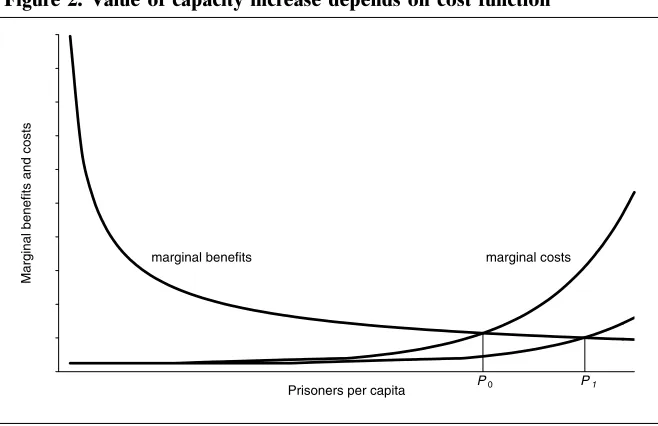
However, we cannot simplify away changes in the prison capital stock. If the supply of state prisons is insufficient by itself to meet demand—specif-ically, if the cost and benefit curves meet at a point after marginal costs have begun to increase rapidly—then it may be beneficial to increase sup-ply (point P0 in Figure 2). The increase in supply would reduce marginal costs, which allows for more prisoners at equilibrium (point P1).
Figure 2. Value of capacity increase depends on cost function
0 0.2 0.4 0.6 0.8 1 1.2 1.4 1.6 1.8 2
Prisoners per capita
Marginal benef
it
s and c
o
s
ts
P1 P0
marginal benefits marginal costs
Prison capacity is notoriously difficult to estimate accurately.15 We can,
however, estimate changes in capacity through the proxy of capital spend-ing on the prison system. Some of this spendspend-ing will no doubt go into deferred maintenance or prison improvements that neither increase beds nor reduce operating costs, but it makes sense to believe that most of it
15. Federal standards allow states to report prison capacity in any of three ways: (1) rated capacity, the expert judgment of an experienced prison official; (2) design capacity, the number of inmates the architect planned for in designing the facility; and
(3) operational capacity, the number of inmates the prison can accommodate while
will go into prison expansion. It may take several years before a project is complete, but eventually most capital spending will shift the cost curve outward, which reduces marginal costs and allows for larger prison populations.
Costs, then, depend on the stock of prison beds available in year 0, plus changes in that stock associated with lagged values of prison capital spend-ing. The number of beds in year 0 is a constant for each state and will be captured by each state’s intercept term (that is, the STATE fixed effect).
Changes can be measured as the summation of the lagged values of capital
spending,
∑
= t
t 0
Kt, where Kt represents annual prison capital spending in
year t. Like prison populations, we can reasonably expect that prison capi-tal spending will respond to values of the other X variables, of the form
Kt = a0 + 1 Xt + ut.
Nevertheless, capital spending in any given year probably depends on expectations of future prison benefits and costs, as measured by the expected values of future predictor variables. Suppose our current expec-tations for future values of Xt (call them Xt*) depend on a simple learning process in which previous expectations are compared with previous actual values. If the actual values are higher than expected, then we adjust future expectations upward; if lower, then we adjust downward. That is,
Xt* –Xt–1* = l (Xt–1 – Xt–1*) (9)
or, equivalently, Xt* is a weighted average of previous actual values and previous expectations:
Xt* = lXt–1 + (1 –l) Xt–1* (10)
If Kt = a0 + a1 Xt–1* + ut, then it is not difficult to show that
Kt* = la0 + la1 Xt + (1 – l) Kt–1 + vt (11) where vt = ut– (1 –l) ut–1. This equation is the standard adaptive
expecta-tions model (Cagan, 1956).
An additional complication is present here, however. Many prison expansion projects take more than 1 year to complete. Our intention is to spend the money necessary to complete the project, Kt*, but because of the complexity of the building process, we can only spend some proportion of that amount in any given year. If that proportion is a constant δ, then it is not difficult to show (Waud, 1966) that Equation 11 can be modified to account for these partial adjustments as follows:
Equation 12 accounts for both mechanical “stickiness” caused by multi-year projects and for adaptive expectations of future need. In practice, we take the logs of K and X to stabilize the variance of v and ensure compara-bility with Equation 6.16
We can expect that the critical predictors of capital spending would be those associated with higher marginal costs: the number of state prisoners in county jails and other institutions, or litigation to decrease crowding in current facilities. A Republican-controlled legislature and a conservative electorate may be more willing to spend limited funds on prisons than on other state functions, which reduces opportunity costs. Capital spending should also depend on funding availability (measured by state revenues net of mandatory expenditures) as well as on expected future increases in prison demand (signaled by increases in crime or social threats or by strict sentencing policies that reduce the state’s ability to control prison popula-tions on a short-term basis). Note that capital spending, like the prison population, could also be put in a benefit-cost form; because we are unable to measure benefits and costs, we are limited to the reduced form of Equa-tion 12.
Thus, we need two equations: a capital spending equation and a more general prison population equation that includes accumulated lags of capi-tal spending.17 The values of predictor variables can affect prison
populations directly (through the prison equation) or indirectly (by affect-ing capital spendaffect-ing, which affects future prison populations through the prison equation). To estimate the full effect of each predictor variable, we need to take both the direct and the indirect effects into account.
16. Use of logs is also likely to improve validity by decreasing the importance of outliers. A purist might reasonably argue that we should be adding values of Kt, not
multiplying them together. This function makes the model much more complicated, however.
17. Capital spending has a significant effect on downstream prison populations for up to 7 years, although the effects diminish as the lag increases. Experimentation showed that a 4-year moving average (that is, the current value plus three lags) pro-duced slightly higher and more significant coefficients than longer lags, and it also allowed for a larger sample size and smaller standard errors on the coefficients for the other variables. The length of the moving average does not have a substantial effect on the results, however.
If capital spending levels affect prison populations on a dollar-for-dollar basis, but we measure changes in population on a proportionate change basis, then we will need to account for steadily increasing prison populations in our definition of capital spending in the prison equation. (If we do not, we are forced to assume that a dollar in capital spending has about four times the effect on prison populations in 2005 as it did in 1977.) The simplest way to do this is to divide spending levels by the previous period’s prison population. Thus, when capital spending enters as an independent variable in the
PRISON equation, it can be considered as a 4-year moving average of capital spending
Estimation
Estimating Equation 8 by ordinary least squares (OLS) is problematic, because log Pt is highly serially correlated and near unit root. As a result, the standard errors of the empirically estimated coefficients for the inde-pendent variables are likely to be greater than they seem, and spurious conclusions may be drawn from the results. If we can reasonably restrict the number of lags in the X variables to one (that is, no Xt–2 is an effective
predictor of Pt), then we can instead rely on the error correction form of Equation 8:
Dlog Pit = bai + bBtDlog Xit – δ (log Pt–1 – bBt–1 log Xt–1) + et (13) The most efficient way to estimate Equation 13 is to estimate an equation of the form:
Dlog Pit = δbai + δbBtDlog Xit– δ log Pt–1 + δbBt–1 log Xt–1 + et (14) which is sometimes called the “single equation” form of the error correc-tion equacorrec-tion. In Equacorrec-tion 14, bBt represents the short-run effect of changes in predictor variables on changes in prison populations, bBt–1
rep-resents the long-run equilibrium effect, and δ remains the speed of partial adjustment. The total effect of a permanent change in independent varia-ble X is equal to bBt (the coefficient on DXt) + bBt–1 (the coefficient on Xt–1
divided by δ). Note, incidentally, that capital spending enters the dynamic portion of Equation 14 as a series of recent annual lags: Skbk log Kt–k (or perhaps as a moving average of annual lags). However, it enters the error correction portion as the sum of all lags from t = 0 to t.
The long-run equilibrium effects are only accurate if the error correc-tion term Pt–1 – bBt–1 Xt–1 is stationary. A complete approach to this
stationarity.18 If we can reject the null hypothesis of unit roots for the
error correction term, then we may reasonably conclude that at least one long-run equilibrium equation exists and that bBt–1Xt–1 is a reasonable
esti-mate of it.
Approach to Inference
This tortuous procedure is likely to lead to a messy result. Each of the 30-odd independent variables enters the prison population twice (once in the dynamic portion and once in the error correction or long-run equilib-rium portion). Each independent variable also enters the capital spending equation. With more than 100 coefficients to be estimated, some are bound to be Type II errors (insignificant predictors that seem to be signifi-cant, just by chance). We can simplify inference and reduce the likelihood of Type II errors by focusing not on individual variables but on classes of competing explanations. Thus, GDP, wage rates, unemployment rates, and poverty rates can all be considered as indicators of a single social threat (a sputtering economy) rather than as separate variables.
To avoid omitted variable bias, let us use a process of backward elimina-tion. All available variables are added to the model; then each category is removed to test the size and significance of the reduction in predictive accuracy. Categories that reduce accuracy the most when removed are presumably the most important predictors. By successively eliminating the least important categories, we can also test the extent to which coefficients for the remaining variables are affected by the stock of variables in the equation, which is a simplified extreme bounds analysis (Leamer, 1983).
Results
Prison Capital Spending Depends on Politics and Resources
Table 3 shows the results of regressions that use all independent vari-ables to predict prison capital spending (that is, estimates of Equation 12). Although the basic model assumes that capital spending will adapt to expected future requirements and only partially adjust from year to year, it is simpler to report short-term effects (that is, lδas, not as). As described, it is not possible to distinguish between expectations effects
(given by l) and adjustment effects (given by δ), but it is possible to deter-mine the product of the two.19 The estimated value of lδ is relatively
precise and varies little among all the specifications considered. Because the long-term effects are the (reported) short-term effects divided by lδ, the long-term effects of a permanent change in any of these variables should be a large multiple (approximately 7.5) of the effects shown.
Table 3. Predictors of P.CAPITAL
OLS Specification Limits
Coefficient Standard error Minimum Maximum
Economic Threat
GDP [–1] 1.534 .871 1.504 2.073
WAGES [–1] 3.921 2.605 2.876 3.903
UNEMP [–1] .539 .256 .478 .627
POVERTY [–1] .099 .133 .079 .130
Underclass Threat
DROPOUT [–1] .452 .271 .397 .486
UNWED [–1] –.083 .501 –.311 .106
FOOD [–1] .464 .292 .419 .550
BLACK [–1] –.098 .259 .101 –.035
HISPANIC [–1] — — — —
Institutional Threat
DIVORCE [–1] –.018 .276 –.071 .010
ENROLLED [–1] 1.994 1.680 1.507 2.727
POLCHANGE –.722 .861 –.777 –.603
MHPOP [–1] — — — —
Public Opinion & Politics
CONSERV .368 .131 .368 .444
REPGOV* –.006 .056 –.029 .004
RCONTROL* .325 .136 .315 .339
MCONTROL* .156 .082 .136 .163
PCTREP .020 .085 .005 .043
19. In Equation 11, only the coefficients on Kt–1 and Kt–2 provide information on l
and δ. Specifically, if a1 is the coefficient on Kt–1 and a2 the coefficient on Kt–2, then a1 = (2 –l–δ) and a2 = – (1 –l)(1 –δ) = lδ–l–δ– 1. Solving both equations for l and
setting them equal to one another leads, eventually, to 0 = δ2
+ (a1– 4) δ + (1 –a1–a2),
OLS Specification Limits
Coefficient Standard error Minimum Maximum
Electoral Cycle
GOVELEC* –.037 .071 –.055 –.021
PRESELEC* .384 .162 .312 .387
CRIME
VIOLENT [–1] .603 .283 .534 .645
PROPERTY [–1] –.752 .684 –.845 –.622
DRUGS [–1] .041 .060 .036 .047
Prison Crowding Conditions
JAIL .044 .021 .038 .050
OTHERINST [–1] .212 .119 .150 .262
LITIGATION* .173 .107 .154 .202
Sentencing Policy
HABITUAL* –.180 .092 –.234 –.137
TRUTH* –.015 .089 –.028 .003
PRESUMP* .160 .109 .146 .184
MJDECRIM* –.241 .090 –.253 –.208
Current Spending
T.SPENDING 5.006 1.211 4.973 6.286
MANDATORY –3.040 .850 –3.597 –3.015
Adjustment & Expectations
P.CAPITAL [–1] .635 .034 .629 .660
P.CAPITAL [–2] –.067 .030 –.087 –.065
Lagged effects (lδ) .134 .018 .130 .143
STATE Fixed Effects
F (49, 1192) 2.253 <.001
YEAR Fixed Effects
c2 (24) 67.744 <.001
R2 .614 — — —
Standard error of residuals .723 — — —
Predictors of prison capital spending are generally consistent with expectations. States spend more when violent crime rates increase (but not property crimes or drug arrests) and when many prisoners are held in county jails and other institutions.20 Capital spending is lower for states
that have decriminalized marijuana and (rather perversely) those that have adopted habitual offender statutes. Presumptive sentencing and truth-in-sentencing policies seem to have little effect on capital spending, however. Some evidence suggests, then, that legislatures respond to an apparent need for prison expansion by increasing capital spending.
Yet other predictors may be more important. Capital spending increases when the electorate is conservative and the legislature is controlled by Republicans (and, to a lesser extent, when one party controls each house). Spending also increases more during presidential election years, when the public presumably is paying more attention. By far, the largest effects are associated with resources. Capital spending increases dramatically with total state spending, and it decreases as more spending is required for edu-cation, welfare, and other mandatory functions.
Little evidence is available to suggest that other social threats matter much. None of the underclass and institutional threat variables is signifi-cant, and the significant increase in spending associated with higher unemployment rates is offset by an increase when GDP increases. The long-term expectations of resource availability may be more at issue here than responding to an economic threat. As shown in the last two columns, none of these coefficients changed much as the specification changed, which suggests that they are also robust with respect to different specifications.21
20. Although crime rates and prison populations seem to be simultaneously deter-mined (see Levitt, 1996; Spelman, 2005; and footnote 24), there is no reason to believe that crime rates and capital spending are simultaneous. Equation 12 and the results shown in Table 3 assume that legislative decisions to increase prison capacity are based on the previous year’s changes in crime rates, not on the current year’s; prison capital spending only translates into capacity increases after a lag. When instruments for vio-lent and property crime rate changes are used in place of the actual changes, the coefficients do not change appreciably.
As noted, prison capital spending seems to respond to expectations of future variables (l seems to be greater than zero), but expectations of future need for prisons do not seem to be particularly important here. The key categories are politics and state spending—not crime, crowding, or sentencing policy. The key expectations, then, are that more prisons will remain good politics, and that the resources needed to pay for them will continue to be available. This finding calls into question the claim that prison capacity increases in response to downstream need for prisons. More on this theory is discussed below.
Long-Run Prison Populations Depend Mostly on Crime and Policy
The prison population model described in this article only holds if a long-term equilibrium relationship exists between PRISON and some
com-bination of the independent variables. This theory is only true if the residuals of the error correction term in Equation 14 are stationary with roots less than 1.0. When Equation 14 is estimated from these data and cross-sectionally augmented Dickey-Fuller tests are applied to these residuals from the 50 states, the average root is .71—the result is moder-ately high but is significantly less than 1.0.22 Because we can reject the
unit-root hypothesis, we may reasonably conclude that the error correc-tion equacorrec-tion represents a long-term equilibrium. Equacorrec-tion 14 thus provides information on both the short-term and long-term effects of each of the independent variables.
on the other variables. Note that the bounds do not measure the effects of changing the variables within categories. Accordingly, more attention should be given to the impor-tance of each category as a whole rather than to the coefficient of any particular variable.
22. More specifically, cross-sectionally augmented Dickey-Fuller tests (Pesaran, 2005) were conducted on the residuals of the error correction term in each state. The average value of the test statistic, t = –1.765, with a standard deviation across states of .735. The null hypothesis of unit root could only be rejected in 2 of the 50 states. Never-theless, the unit-root test results are homogeneous. That is, they are consistent with the hypothesis that the root for all residuals is the same; c2
50 = 41.232, p(c2) = .807. Thus, a
panel test (Im, Pesaran, and Shin, 2003) is appropriate. The panel test result,
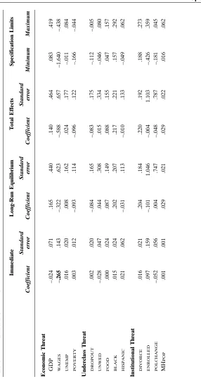
Table 4 shows the estimates. The first two columns show the short-term effects (bBt, the coefficients on the DXt variables) and their standard errors. Columns 3 and 4 show the long-term effects (bBt–1, the coefficients
on the Xt–1 variables divided by –δ, the coefficient on PRISONt–1) and their
standard errors. Columns 5 and 6 show the total effects (bBt + bBt–1) and
standard errors. As it happens, the distinction between short-term and long-term effects is important for some of these variables.23
Some variables have a significant impact on PRISON in the short run but
not in the long run. Previous capital spending (our proxy for increased prison capacity) and current state spending (net of spending on mandatory functions) clearly affect annual changes in prison populations in the expected (positive) direction. However, they do not seem to have long-term effects. Thus, capacity and funding affect the timing of prison popula-tion increases: Populapopula-tions only increase when the beds and the money are available. But sooner or later, they will be available.
Other variables affect prison populations in both the short run and the long run. Crime rates are a clear example. In the short run, prison popula-tions seem to increase as drug arrests increase and property crimes decrease. This result is unexpected, but it can be explained by the counter-vailing effects of prison on crime rates. We can be sure that prisons reduce crime, at least to some extent (cf. Levitt, 1996; Western, 2006). If increases in crime also lead to increased prison populations, the apparent short-run effects of violent and property crime rates as well as (perhaps) drug arrests would be a mixture of these two effects. The figures shown in Table 4 are consistent with this hypothesis.24 If the effects of prison on crime are
23. When the equation is restricted to short-term effects only, eliminating the error correction term, the short-term effects are very similar to those shown in Table 4. Only for one variable does the restricted equation provide an estimate of short-term effects that differs by as much as one standard error from the short-term estimate pro-vided by the unrestricted equation. That variable, HISPANIC, is marginally significant in
the restricted equation (bBt = –.108, one-tailed p≈ .042) and not significant in the error
correction model.
24. The best way to account for simultaneity is to replace the simultaneous inde-pendent variables with instruments. In this context, these instruments are predictions of what violent and property crime rates would have been if prison populations had not increased (and presumably reduced crime rates through incapacitation and deterrence). To obtain these instruments, we need to find variables that predict crime rates but do not have any effect at all on prison populations and can be excluded from the PRISON
equation.
T
a
ble 4. Pr
Immediate Long-Run Equilibrium T otal Effects Specification Limits Standard Standard Standard Coef ficient error Coef ficient error Coef ficient error Minimum Maximum
Public Opinion & P
Immediate Long-Run Equilibrium T otal Effects Specification Limits Standard Standard Standard Coef ficient error Coef ficient error Coef ficient error Minimum Maximum Curr ent Spending T . SPENDING .250 .082 – .172 .486 .078 .549 – .158 .381 MANDATORY – .116 .070 .446 .480 .331 .519 .144 .621 P
artial Adjustment PRISON
[–1 ] – .120 .019 — — — — – .121 – .105 F ixed effects STATE
: F (49, 1160)
2.838 <.001 — — — — — — YEAR : c
2 (23)
109.968 <.001 — — — — — — Long-Run Equilibrium F (33,1160) 2.538 <.001 — — — — — — R 2 .367 — — — — — — —
Standard error of residuals
.053 — — — — — — — Notes . T
his table shows coefficients and heteroskedasticity- and autocorrelation-consistent standard errors. All continuous variable
s except
P
.
CAPMA
are logged and differenced;
P
.
CAPMA
is logged but not differenced. Dummy variables are denoted by an asterisk. T
he coefficients for continuous
variables are elasticities; the coefficients for dummy variables show proportionate change in prison population associated with
presence of
characteristic. Statistically significant coefficients (
p
< .05, one-tailed test) are shown in
bold
. Specification limits show the minimum and maximum
coefficients obtained over 19 regressions with one or more categories deleted. All models use 1,300 observations and include fi
xed
YEAR
and
STATE
mostly short run in nature, however, we can expect these countervailing effects to be much less apparent in the long-run estimates. Indeed they are: In the long run, prison populations increase as violent and property crime rates as well as drug arrests increase (although only the violent and drug effects are statistically significant). The net result of the short-run and long-run effects is positive.
Sentencing policies also seem to have both immediate and long-run effects in the expected directions. Presumptive sentencing and marijuana decriminalization reduce prison populations in both the short run and the long run. Truth-in-sentencing laws have little immediate effect but a sub-stantial long-run effect. This analysis makes sense: Truth-in-sentencing laws increase time served and reduce the number of offenders released in future years; the full effect would only be observed after prisoners sen-tenced under the old regime are replaced by those sensen-tenced under the new law. Habitual offender laws seem to have little effect at all, perhaps because they only affect the sentences of a small number of offenders (Zimring, Hawkins, and Kamin, 2001).
(the proportion of the population who are less than 15 years old or older than 65) and especially high risks (military personnel, recent migrants to the state, tourists), and, for property crimes, the extent of social cohesion (proxied by the suicide rate). When these variables are used to predict crime rates, the increase in R2
is highly significant (F for violent crimes is about 14, for property crimes about 12, both with p < .001), but these variables are not significant predictors of prison populations F(7,1185) = .905 in the capital spending equation and F(7,1181) = .986 in the prison equation, neither of which approaches statistical significance). When the instruments are used in place of actual violent and property crime rates, the short-run coefficient in the prison equation changes from .024 [.028] to .211 [.133] for violent crimes, and from –.098 [.043] to –.023 [.264] for property crimes. Neither of these coefficients is statistically significant, but they change in the expected direction and are reasonable in size. Using instruments for short-run crime effects also has very little effect on the short-run effects of drug arrests or on any of the long-run coefficients. We may reasonably conclude that violent crimes have a substantial, positive effect on prison populations in the long run and may also have a positive effect in the short run, and that property crime rates have essentially no short-run effect on prison populations, although they may have a substantial long-run effect. Thus, the negative coefficient for property crimes in Table 4 is probably caused by simultaneity, and not by any real effect of crime rates on prison populations. Although Table 4 shows the natural variable estimates rather than the instrumental estimates, the analysis of Table 5 is based on the instruments. This result has the practi-cal effect of reducing the apparent importance of crime rate changes. Using actual crime rates and not instruments leads to a higher change in R2
The most important results here may be the dogs that do not bark. A conservative electorate and a Republican legislature are more likely to increase capital spending and subsequent availability of prison space, but they do not seem to have any direct effect once capital spending has been taken into account. Crowding behaves much the same way: It affects populations only through capital spending. Prison populations, like capital spending, do not seem to respond at all to economic threats, underclass threats, or institutional threats.
The autoregressive term (the coefficient for PRISONt–1 in Table 4) is very
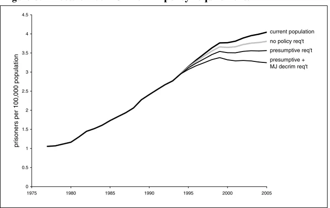
low at –.120, which means that only a small fraction of the deviations from long-run equilibrium is corrected in any given year. If none of the inde-pendent variables changed at all, it would take 5 or 6 years for prison populations to move even 50% of the way toward the long-run equilib-rium value, depending on the specification. It would take 12 to 15 years to move 80% of the way. This result is consistent with the limited response of prison populations to the crime decrease of the 1990s. The crime decrease was offset by increases in use of truth-in-sentencing laws, and the move-ment toward the lower, long-run equilibrium value has been very slow.
Crime and State Spending Are the Best Predictors of Prison Population
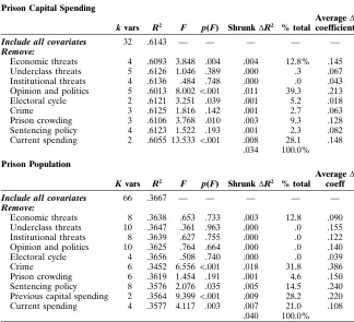
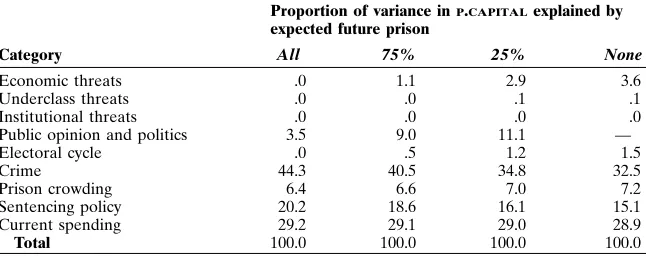
Judging from the coefficients alone, the story looks fairly complicated. Many variables—which represent a wide variety of social, political, and economic explanations—seem to be related to prison capital spending or populations. It is difficult to tell which are most important. One way to estimate the relative importance of each of these explanations is to observe what happens when we remove variables from the model, one category at a time. R2 values will decrease, of course; we can measure the
significance of this reduction (and thus the value of including each cate-gory in the complete model) through an F statistic. We can also compare the reductions in R2 across categories, shrinking the values toward zero to
reduce capitalization on chance (Box and Tiao, 1972). The proportion of the total R2 accounted for by each category provides a rough estimate of
that category’s importance. This estimate can be misleading if two or more categories are collinear; in this case, eliminating one category may affect the size and significance of the variables in the remaining categories. If the coefficients do not change by much, we can be fairly sure that the change in R2 is measuring the effect of the removed category.
spending are statistically significant, but crime and previous capital spend-ing—more or less, current prison capacity—seem to explain more than the others. In no case did removal of a category appreciably affect the remain-ing coefficients, so we can be fairly certain that these estimates are untainted by collinearity across categories.25
Capital spending is an intervening variable in this analysis. It does not itself cause prison populations to increase, but it makes future increases possible. Thus, the other variables affect prison populations in two ways: directly (in the prison equation) and indirectly (by affecting capital spend-ing, which affects future prison populations). When direct and indirect effects are combined, eliminating current capacity as an explanation, the critical categories are crime and state spending, followed by sentencing policy, politics, and crowding. That is, the principal drivers of prison popu-lations are the apparent need for more prisons and the ability to pay for them. Politics matters, too, but not as much. Other social threats do not matter at all.
25. The size of the differences were measured in three ways: (1) the absolute value of the difference in coefficients between the complete model and the removal model, divided by the standard error of that coefficient in the complete model; (2) the number of coefficients that change by as many as one standard error when some category of variables is removed; and (3) the number of coefficients that change in statistical signifi-cance (that is, from insignificant to significant or vice versa). The removal of several categories changed the significance of the remaining coefficients because several vari-ables in the complete model were marginally significant or marginally insignificant. However, only two coefficients changed by as much as a single standard error. (The long-run equilibrium coefficients on WAGESand MHPATIENTSin the PRISON equation
Table 5. Relative importance of independent variables in explaining prison capital spending and population
Prison Capital Spending
Average D k vars R2 F p(F) Shrunk DR2 % total coefficient
Include all covariates 32 .6143 — — — — —
Remove:
Economic threats 4 .6093 3.848 .004 .004 12.8% .145 Underclass threats 5 .6126 1.046 .389 .000 .3 .067 Institutional threats 4 .6136 .484 .748 .000 .0 .043 Opinion and politics 5 .6013 8.002 <.001 .011 39.3 .213 Electoral cycle 2 .6121 3.251 .039 .001 5.2 .018
Crime 3 .6125 1.816 .142 .001 2.7 .063
Prison crowding 3 .6106 3.768 .010 .003 9.3 .128 Sentencing policy 4 .6123 1.522 .193 .001 2.3 .082 Current spending 2 .6055 13.533 <.001 .008 28.1 .148
.034 100.0%
Prison Population
Average D K vars R2 F p(F) Shrunk DR2 % total coeff
Include all covariates 66 .3667 — — — — —
Remove:
Economic threats 8 .3638 .653 .733 .003 12.8 .090 Underclass threats 10 .3647 .361 .963 .000 .0 .155 Institutional threats 8 .3639 .627 .755 .000 .0 .122 Opinion and politics 10 .3625 .764 .664 .000 .0 .140 Electoral cycle 4 .3656 .508 .740 .000 .0 .039
Crime 6 .3452 6.556 <.001 .018 31.8 .386
Prison crowding 6 .3619 1.454 .191 .001 4.6 .150 Sentencing policy 8 .3576 2.076 .035 .005 14.5 .240 Previous capital spending 2 .3564 9.399 <.001 .009 28.2 .220 Current spending 4 .3577 4.117 .003 .007 21.0 .108
.040 100.0%
Notes. This table shows the effects of removing one category at a time from the complete model. Shrunk DR2 = (1 – 1/F removal)(R2 complete – R2 removal). “% total” is an
approximate share of explanatory power associated with each category. “Average D coeff” is an average difference between complete and restricted model for remaining coefficients, measured in standard errors.
Discussion
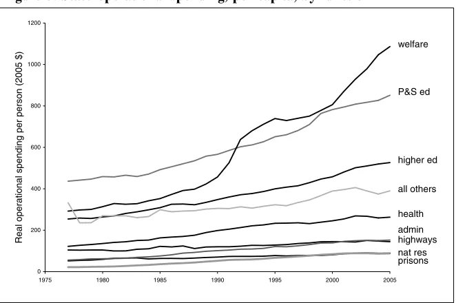
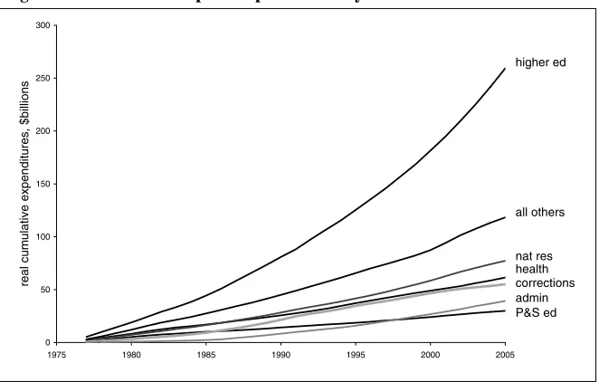
Some of these findings are expected. It comes as no surprise to find that prison populations increase with prison capacity or crime rates, or in response to more or less punitive sentencing policies. However, the impor-tance of state financial resources—explaining nearly 30% of the total variation in prison populations—may be surprising. How can money be a cause of our problem? Wouldn’t this affect everything else that states do, too? Of course it would. It did. As Figure 3 shows, spending increased for all state functions between 1977 and 2005. The prison increase was higher than for most other functions: Spending on prison operations quadrupled (as did prison populations); operational spending on primary and secon-dary education, higher education, and health only doubled. Nonetheless, all boats rose with the tide of cash.
Figure 3. State operational spending, per capita, by function
0 200 400 600 800 1000 1200
1975 1980 1985 1990 1995 2000 2005
Real operational spending per person (2005 $)
welfare
P&S ed
higher ed
all others
health