Influence analysis of sprinkler irrigation effectiveness using ANFIS
Zhongwei Liang
1,2,3*,
Xiaochu Liu
1,2,3,
Guilin Wen
2,
Xuefeng Yuan
3(1. Guangdong Engineering Research Centre for High Efficient Utility of Water/Fertilizers and Solar Intelligent Irrigation, Guangzhou University, Guangzhou 510006, China;
2. School of Mechanical and Electrical Engineering, Guangzhou University, Guangzhou 510006, China; 3. Advanced Institute of Engineering Science for Intelligent Manufacturing, Guangzhou University, Guangzhou 510006, China)
Abstract: In order to improve sprinkler irrigation quality and promote actual irrigation efficiency, the influence analysis of sprinkler irrigation effectiveness (SIE) using ANFIS (Adaptive Neural Fuzzy Inference System) was implemented to balance moisture infiltration and water redistribution in soil field. Firstly, using a detailed description of governing equations proposed for sprinkler irrigation flow, the theoretical foundation and mathematical model of irrigation effectiveness can be established; Secondly, based on a complete preparation of experimental irrigation conditions, a series of calibration indexes quantifying SIE for sprinkler irrigation quality and infiltration efficiency were proposed; Then thirdly, a novel ANFIS system was designed and introduced to evaluate these key effectiveness indexes in actual working operations, so that a series of detailed influence analysis and comprehensive infiltration assessment focusing on sprinkler irrigation effectiveness could be achieved afterwards, which result to the realization of better infiltration equilibrium and higher water redistribution efficiency in actual irrigation test. Therefore, the qualification of sprinkler irrigation effectiveness was achieved, and in addition, the moisture infiltration improvement and soil moisture uniformity were facilitated also in return.
Keywords: influence, analysis, sprinkler irrigation, effectiveness, ANFIS DOI: 10.25165/j.ijabe.20191205.5123
Citation: Liang Z W, Liu X C, Wen G L, Yuan X F. Influence analysis of sprinkler irrigation effectiveness using ANFIS. Int J Agric & Biol Eng, 2019; 12(5): 135–148.
1 Introduction
Sprinkler irrigation has been widely employed throughout China due to water shortage, environmental protection, and frequent droughts, thus the irrigation effectiveness deserves high attentions to promote its working capability. In this research, the concept of sprinkler irrigation effectiveness (SIE) is defined as the distributive equilibrium of sprinkling moisture infiltration in soil field, which facilitates the balanced cultivation of crop plant and depends on the complicated interrelation mechanism between experimental conditions, flow properties and irrigation implementations. As sprinkler irrigation saves more than half of water resource compared with other alternative approach does, meanwhile it is appreciated by such superiorities as equilibrium infiltration distribution, cost saving and user friendly, which make it be frequently used in agricultural cultivation or city landscaping. Since moisture infiltration equilibrium in soil field is highly emphasized to improve irrigation efficiency, its inherent characteristics should be studied thoroughly, including the infiltration rate, average water irrigation efficiency, transpiration losses, and the infiltration depth of soil ground, etc. Furthermore,
Received date: 2019-05-13 Accepted date: 2019-09-15
Biographies: Xiaochu Liu, PhD, Professor, research interests: intelligent agriculture equipment and high-performance irrigation engineering, Email: [email protected]; Guilin Wen, PhD, Professor, research interests: agriculture engineering, Email: [email protected]; Xuefeng Yuan, PhD, Professor, research interests: intelligent control of irrigation equipment, Email: [email protected].
*Corresponding author: Zhongwei Liang, PhD, Professor, research interests: agriculture engineering and intelligent precision irrigation. School of Mechanical and Electrical Engineering, Guangzhou University, Guangzhou 510006, China. Email: [email protected], [email protected].
the coefficient of infiltration equilibrium is also treated as an important factor relates to irrigation management. Based on these definitions a comprehensive influence evaluation on irrigation network and working schedule would be realized, meanwhile the promotion of irrigation effectiveness could be facilitated, too.
Recently, more researches provided theoretical foundations and scientific supports to study the irrigation water allocation and infiltration effectiveness in actual experiments. For instance, a series of investigations have been proposed already on the efficient water-allocation model and economic optimization of irrigation capacity[1-6], a beneficial and sustainable management of water
distribution and infiltration efficiency for the irrigation project of Nile Basin has been analyzed[7]. Simultaneously, Hellín et al.[8] and
Opan et al.[9] respectively reported their instructive studies of
irrigation effctiveness improvement using the DPSA-based (Dynamic Programming Successive Approximation) optimization model. More studies concerning the irrigation effectiveness schedule, and the effect of subsurface drip irrigation compared with that of surface drip irrigation, can be summarized from literature[10,11]
accordingly. Relevant researches focusing on the upgrading of supplemental irrigation effectiveness for wheat production are published in literature[12], either. It should be pointed out that a
detailed and systematic analysis focusing on the irrigation effectiveness of water distribution, rather than a traditional macroscopic irrigation management characterized by purely parametric testing and simply production monitoring, should be investigated in the near future for the upcoming research developments of irrigation effectiveness in accuracy and reliability undoubtedly.
To optimize the infiltration effect of sprinkler irrigation, literatures[13-15] demonstrated their innovative developments on the
et al.[16] mapped the annual effectiveness area of crop cultivation in
one specific irrigation district by applying a classifier of plant phenological index; Bargués et al.[17] and Nasiakou et al.[18]
discussed on the parameters of filtered volume and flow outlet in drip irrigation occasions, and the subsurface drip effects for smart irrigation as well. More progresses on this subject could be learned from literatures[19-23] also. As some scholars began paying
their endeavour on the quantitative evaluations of sprinkling effectiveness, Leduc et al.[24] presented some suitable and optimal
effectiveness evaluation indexes to assess the photovoltaic water pumping efficiency for grassland irrigation; Garga et al.[25]
proposed an integrated irrigation effectiveness model characterized by non-linear calculative function in the hope of obtaining the optimum cultivation pattern and reasonable irrigation schedule for deficit irrigation.
Since sprinkler infiltrate capability is very difficult to be quantified directly, Koech et al.[26] made a real-time infiltration
monitoring for irrigation effectiveness; A novel architecture of wireless sensors for wetting effectiveness monitoring can also be found[27,28] recently; Furthermore, Yang et al.[29,30] and Rufat et
al.[31] have focused on the effectiveness equilibrium state of
sprinkling water allocation as well. To model the pulsing impact of irrigation drip effectiveness, Phogat et al.[32] made a detailed
work report. Furthermore, as fuzzy system provides a high-efficient method to calibrate irrigation quality[33], Montesinos
et al.[34] tested the design of ANFIS for the optimization of energy
cost in a pressurized irrigation network. Moreover, Alison et al.[35]
demonstrated their recent achievements on the control strategies for irrigation planning by using fuzzy reasoning. Somehow, few published literatures focused on the employment and improvement of ANFIS to study irrigation effectiveness in the past several decades; some existing problems concerning with their quantitative evaluations and mutual- influence mechanisms remain unsolved, so that a systematic research on this topic should be focused and upgraded.
In order to realize the accurate influence analysis of sprinkler irrigation effectiveness using ANFIS, the next section gives the governing equations of irrigation flow and droplet infiltration; as Section 3 prepares for the test environment and sprinkler irrigation systems, Section 4 describes actual sprinkler irrigation processes in details; thereafter Section 5 makes a thorough influence analysis of sprinkler irrigation effectiveness, in the end Section 6 concludes this research comprehensively.
2 Governing equations
The water jetting relevant to sprinkler irrigation starts from water droplet exiting from the orifice of sprinkler nozzle and ends when the sprayed droplets are formed. An applicable sprinkler emits water droplets by which droplet formed in the orifice, then droplet travels independently until it reaches soil ground and can be measured precisely by the array of tensionmeter. In a typical testing condition, the linear distance between the landing point of water droplet and the nozzle orifice could be regarded as a linear function of droplet diameter. The theory of ballistic motion is frequently used to calculate the moving path of jetting droplet considering its initial status and external force influence. Gravity acts on the vertical direction of soil ground, in addition air resistance assumed as opposite to the moving direction of droplet trajectory, which produce a composite force acting on water droplet. Therefore, the droplet motion velocity towards soil ground keeps
equal to the vector composition of water jetting speed in air ambience and wind speed. To give the governing equations of irrigation flow and droplet infiltration, some assumptions should be made in advance: water flow departing from nozzle exit is disintegrated into scattered water droplets, and they projected respectively into air ambience accompanied by Reynolds drag coefficient, which separates from key environmental variables such as the sprinkler height over soil field, trajectory angle of jetting flow, speed of wind, diameter of nozzle, and other influential factors; Every water droplet projected to different distance and impacts on field zone without interacting with each other. So that in order to quantify the mathematical model of irrigation flow and droplet infiltration, during the complete trajectory process of droplet flight, by considering the integrated actions of gravity, buoyancy forces and resistance, it could be described as [33-35]:
2
2
3 ( )
4
a D
x x
w
d x ρ C υu w
dt = − ρ D −
2
2
3 ( )
4
a D
y y
w
d y ρ C υu w
dt = − ρ D −
2
2 3 4
a D a w
z
w w
d z ρ C ρ ρ
υu g
dt ρ D ρ
−
= − + (1)
where, x, y and z are the three-dimensional coordinate values (mm) of objective water droplet in the air, with the origin point of its trajectory path positioned at the orifice exit; D is droplet diameter;
ρa is air density, g/mm3; ρw is density of water, g/mm); u denotes its
flight velocity, mm/s; ux, uy, uz stand for the speed components in three coordinate directions, mm/s; v is the relative droplet speed , mm/s; g is gravitational acceleration, mm/s2; Re is Reynolds
number; υ is the air viscosity coefficient; CD is air drag coefficient; w is wind speed, mm/s; and wx, wy are its two components in x and y axis, mm/s. Here the drag coefficient of sprayed droplet depends on Reynolds number and slip velocity is:
| |
e a
u w D
R ρ
υ
−
= (2)
where, drag coefficient can be determined by the following correlations:
0.687 (1 0.15Re ) 24
e D
R C =⎛⎜ ⎞⎟ +
⎝ ⎠ (3) Wind speed can be calculated by:
0 0
( ) ( )ln z hr ln za hr
w z w a
z z
− −
⎛ ⎞ ⎛ ⎞
= ⎜ ⎟ ⎜ ⎟
⎝ ⎠ ⎝ ⎠ (4) where, w(z) is the wind velocity relates to the orifice height z, mm/s; w(a) is the measured one at the orifice height za, mm/s; hr is the height of plant and z0 is the referential height of soil ground, mm. Thus the mathematical model calibrating the change of droplet
diameter can be demonstrated as[24,36]: Δ
2 v a
u
m w f
dD M K ρ PN
dt = − M Dρ P (5) where, Mv is vapour molecular weight; Mm is the mean weight of water-gas mixture; K is the diffusivity of vapour, mm2/s; and Td is
the temperature of sprinkling water, °C; Furthermore, ΔP describes the difference between saturation pressures, kPa; Pf is air pressure, kPa; and Nu is Nusselt number. The initial diameter of water droplet is set by 0.5 mm, so that its heat-balance equation could be demonstrated as[23,35,36]:
dt dM L q dt dT C
M d v
D
where, Nu=2+0.6Re1/2Pr1/3. Based on this prearrangement the SIE level (Sl) on the irrigated soil filed can be determined as:
c p av M c
l HW S F H
S = / + for t>tp (7)
where, Hc is soil hydraulic conductivity; Sav is water pressure; Fp is
field infiltration rate; WM is water deficit; Fp can be determined as:
0
( ) ln(1 / )
c p p M av p M av
H t t− +t =F −W S +F W S for t>tp (8)
where, t is current time; tp is the specific time for irrigation measurement and can be determined as
/ ( )
p c M av r c r
t =H W S P −H P (9) where, Pr is the precipitation amount of sprinkler irrigation, mm; t0
is the time scale shift due to cumulative infiltration rate for irrigation measurement, which can be calculated as[28,36]:
0 p M avln 1 p
c c M av
F W S F
t
H H W S
⎛ ⎞
= − ⎜ + ⎟
⎝ ⎠ (10) Based on these governing equations the irrigation flow and droplet infiltration could be described.
3 Test preparation
3.1 Experimental environment
The sprinkler irrigation experiment was implemented in the greening district of Guangzhou University, where the large-scale water irrigation is started systematically after the completion of university campus (23°03′1.23″N, 113°24′3.92″E) in 2004, which locates at the southeast part of Guangzhou city. This area is mainly covered by hills or fluvial plain, hilly area locates at the central region with the slope angled by 20º-30º, and fluvial plain by the elevation height of 40 m. Its hilly area shows good quality of soil texture but full of silt or liquefiable sandy featured by water-saturation, high porosity and compressibility. The campus of Guangzhou University possesses a perfect environment of natural ecological vegetation and surrounded by the shore of Pearl River, which imposes positive influence on the greenery irrigation and establishment of scenery ecosystem. Guangzhou lies at the sub-tropical zone of China, characterized by the mean annual temperature of 21.5℃-22.6 , precipitation of 1623.6℃ -1899.8 mm, and evapotranspiration of 1603.5 mm, according to the weather records of the past 60 years taken from Guangzhou meteorological agency. It is also noteworthy that Banyan, Kapok, Bauhini a, Dalbergia hupeana, Hemp palm, Magnolia, Chinese wistaria, Zoysia matrella, Nephrolepis biserrata, Arachis duranensis, and Rhododendron, are widely distributed in this area.
The greening field sized by 200 hm2 and the sprinkler
irrigation was implemented every day between 8:00am and 4:00pm from June 5th to September 2rd, 2018. Table 1 presents the ground
elevations of key nodes in the targeted irrigation network, here the diameters of main and branch pipes are sized by 50 mm and 40 mm respectively, and the total length of irrigation pipeline reaches 400 m. The organic content measured from different soil layers by the depth in 0-500 mm is 22.60 g/kg, nitrogen content is 1.68 mg/kg, density of soil bulk is 1.39 g/mm, field capacity is 26.3%, and soil pH is 6.75. A tested area squared by 50.0 m× 20.0 m is separated from its surrounding field by using PVC plates inserted to soil field by the depth of 0.5 m, to prevent the possible seepage of irrigation water nearby. After a series of detailed testing considerations and plant habit comparisons Zoysia matrella was selected out as the experimented plant for its extraordinarily tolerance of high salinity and robust adaptation capability, making it ideal for infiltration observation and growth control in soil field,
simultaneously a frequently-used method of ridge cultivation is used to make the influence analysis of SIE.
Table 1 Ground elevations of key nodes in the experimented irrigation network (m)
1 2 3 4 5 6 7 8 56.5 56.3 56.8 57.3 56.5 58.2 58.2 57.1
9 10 11 12 13 14 15 16 57.8 58.7 59.2 60.5 60.3 58.5 56.6 57.8 3.2 Sprinkler system
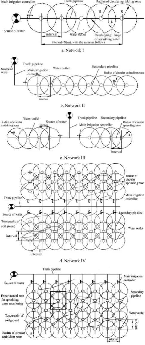
After repeatedly project selections and structural adjustments, typical layout types of irrigation networks labeled from I to V are illustrated by Figures 1a-1e with respect to the specific topographic condition, lifting position, border type, farming type, wind speed, wind direction, and the border length of irrigation field, thus they could be prepared and arranged for sprinkler irrigation test and the influence evaluation of irrigation effectiveness. As these tested networks are arranged at a well-irrigated area, the vertical height of their sprinkler nozzle is 80 mm, and the wetting diameter overlap of 55%-60% should be ensured, according to the specific environmental requirements of geographic area and plant species, and the comprehensive consideration of ground topographic features. In Figure 2 the experimented soil field to be irrigated is divided into many meshed grids by identical areas, therefore actual irrigation effectiveness caused by different irrigation networks can be investigated and compared, meanwhile five layers segmented from different soil depth of 0-500 mm for infiltration measurement are described also. This sprinkler irrigation system is come up with by integrating the high-efficient fluid intensifier pump, revolving sprinkler nozzle, and sprinkling water monitoring system consisted by precision tensionmeters together, so Figure 3 demonstrates the on-site layout of sprinkler irrigation network currently used. As the intensifier pump supplies water up to a maximum pressure of 500 kPa, so that irrigation water can be pressurized into sprinkler nozzle and stabilized by accumulator. But in this experiment a much lower pressure of 300 kPa would be used by the revolving sprinkler nozzle to make sure that the wetting depth of soil field can be measured and controlled more easily, meanwhile the concentration of sprinkling water can be maintained constantly, too. The filtrated water is forced into a nozzle orifice that makes the jet travels throughout sprinkler body in high speed to create a partial vacuum in the inlet of water droplet. The irrigation time can then be recorded and extended until a generally-steady rate of moisture infiltration is obtained. Table 2 gives some representative environmental conditions of sprinkler irrigation for guidance, including the jetting pressure in nozzle orifice (P, kPa); irrigation time (IT, h); amount of sprinkling water discharge (Q, L/h); average value of air temperature (T, °C); average value of air relative humidity (RH, %); average wind speed (U, m/s); and direction (WD) as well.
the calculation of sediment yield, the mean radial distribution of sprinkling water is measured in a calm environmental condition, the pressure and velocity of jetting flow are monitored and controlled on-line via signal acquisition with the help of a computer workstation, which comprised by Intel core i9 7900X microprocessor, Matlab R2018b, and Windows 10, so that the computer-controlled monitoring system for SIE analysis could be established for the measured data from actual irrigation experiments.
a. Network I
b. Network II
c. Network III
d. Network IV
e. Network V
Figure 1 Typical layouts of irrigation networks labeled from I to V
Figure 2 The planar distribution of infiltration tensiometers at the experimental irrigation area for sprinkling water monitoring
Figure 3 On-site layout of sprinkler irrigation network Table 2 Environmental conditions
No. P/kPa IT/h Q/L·h-1 T/℃ RH/% U/m·s-1 WD 1 280 2.0 1356 26.5 82 1.5 NW 2 300 2.5 1457 28.6 88 1.0 SE 3 315 2.3 1517 30.2 76 0.8 N/NE 4 328 2.8 1526 31.5 92 0.6 N 5 365 2.6 1547 28.9 78 1.1 E/SE 6 380 3.0 1488 29.5 85 1.2 ES 7 246 2.5 1492 28.7 86 0.8 NE 8 360 2.5 1687 32.5 77 0.9 NE 9 258 2.0 1852 33.1 72 0.5 S/SE 10 348 2.2 1725 28.6 82 1.3 S 11 338 2.4 1744 34.5 65 1.1 SE 12 364 2.6 1795 30.2 62 1.0 E/NE 13 275 2.5 1896 28.6 63 0.8 E 14 384 2.3 1855 27.7 80 0.6 NE 15 300 2.5 2025 28.7 58 0.5 NW 16 386 2.8 2014 26.9 82 0.7 SE 17 357 3.2 1933 30.5 71 0.9 S/SE 18 264 3.0 1856 28.6 73 1.0 S/SW 19 350 3.0 1875 27.8 83 1.2 N 20 378 2.5 1864 29.5 80 1.0 N/NW 21 310 2.3 1859 26.8 85 1.2 S 22 305 2.5 1875 27.8 79 0.8 SE 23 312 3.0 1859 28.8 90 0.7 E/N 24 285 3.1 1925 32.5 91 0.5 E 25 337 2.5 1922 31.5 82 0.6 W/NW 26 358 2.4 1845 30.5 73 0.4 W 27 257 2.6 1752 32.6 80 1.2 NW 28 364 2.5 1773 33.4 72 1.2 SW 29 354 2.4 1859 34.4 74 1.1 SW 30 267 2.5 1902 29.5 77 0.6 N 31 368 2.4 1856 30.5 83 0.5 N 32 270 2.8 1854 32.6 86 0.5 W/SW 33 384 3.1 1847 26.9 82 0.8 SW 34 392 2.6 1856 25.4 84 0.9 SW
...
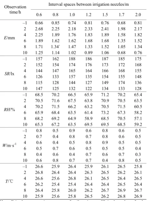
Table 3 The measured values of moisture evaporation and meteorological factors in different interval distances
Observation time/h
Interval spaces between irrigation nozzles/m
0.6 0.8 1.0 1.2 1.5 1.7 2.0
E/mm
–1 0.66 0.85 0.74 0.81 0.76 0.68 0.81 2 2.68 2.25 2.18 2.33 2.41 1.98 2.17 4 2.25 1.89 1.76 1.83 1.89 1.58 1.82 6 1.89 1.62 1.62 1.68 1.68 1.35 1.52 8 1.71 1.34` 1.47 1.33 1.52 1.05 1.34 10 1.25 1.14 1.02 0.89 1.06 0.68 0.76
SR/lx
–1 157 162 188 186 187 185 175 2 152 154 174 176 173 172 168 4 144 147 165 164 166 168 155 6 126 133 157 135 154 155 148 8 115 128 144 127 149 174 136 10 147 125 132 122 134 133 128
RH/%
–1 68.5 70.2 66.5 65.9 71.2 70.2 65.4 2 70.5 71.6 67.5 63.8 70.9 70.5 63.5 4 70.2 71.5 66.2 63.2 70.5 71.5 60.5 6 65.9 68.4 63.5 61.4 73.2 67.3 58.2 8 68.2 69.2 64.9 58.9 68.5 70.5 57.1 10 65.3 67.2 63.5 69.5 69.5 68.5 59.2
W/m·s-1
–1 0.8 0.5 0.9 0.6 0.8 0.6 0.5 2 0.7 0.4 0.8 0.7 0.8 0.6 0.5 4 0.6 0.4 0.5 0.8 0.9 0.5 0.5 6 0.5 0.7 0.6 0.5 0.5 0.5 0.4 8 0.4 0.6 0.4 0.7 0.6 0.7 0.3 10 0.6 0.8 0.7 0.7 0.4 0.8 0.5
T/℃
–1 26.6 25.9 26.4 25.9 26.1 26.5 25.8 2 26.8 26.4 26.4 26.3 26.5 26.2 26.1 4 26.6 25.6 26.8 26.1 26.5 26.4 26.5 6 26.2 25.4 25.4 26.4 26.4 26.5 26.4 8 26.4 25.8 26.0 26.2 26.7 26.9 26.7 10 25.9 25.6 25.8 26.5 26.2 26.8 26.9 Here E is the evaporation amount of soil moisture; SR is the value of solar radiation; RH is air relative humidity; W is wind speed; T is air temperature; –1 h, 2 h, 4 h, 6 h, 8 h, 10 h denote the specific time point of process monitoring for sprinkler irrigation.
4 Experiment
Since an accurate description and detailed investigation of irrigation effectiveness influence still kept in an undeveloped state[40], due to the absence of efficient effectiveness evaluation for
their mutual correlation, sprinkler irrigation should be improved through the monitoring of flow properties and the implementation of influence analysis. As Figure 4 presents the tested zone for water sprinkling correction, with the dramatic developments of computer processing power, computational fluid dynamics (CFD) is utilized here to study the detailed knowledge of prediction and evaluation of sprinkler irrigation effectiveness. In order to reveal the precipitation amount and moisture infiltrate situation in soil filed, numerical simulation has been conducted as Figure 5 shows. Thereafter a set of actual experiments can be carried out under the guidance of CFD simulation, to evaluate the obtained results and influential mechanism of sprinkler irrigation.
As we all know that, sprinkler irrigation is a complicated process in which a bunch of high-pressure sprinkling stream experiences radical and instantaneous changing state caused from different conditional factors[41,42], some typical flow properties are
therefore applied as the crucial factors for irrigation effectiveness analysis: RMS Velocity (Rms), Turbulence Intensity (Ti), Turbulence Kinetic Energy (Tc), Turbulence Entropy (Te) and Reynolds Shear Stress (Rs), since they present an accurate and reliable calibration of irrigation effectiveness[40,43,51]. Firstly their
reference levels could be determined, with the selected calculation scheme of sprinkling water distribution and infiltration
effectiveness, the constructive influences caused by these flow properties on the working capability of sprinkler system are thereby compared with. The change range of our influence investigation occupies more than 95% of their reference levels, so that it covers almost all of the possible values of these flow properties.
Figure 4 Tested zone for water sprinkling correction
Figure 5 Infiltration effectiveness level on irrigated soil ground
a. The meshed grid established to calibrate the levels of droplet infiltration at different coordinate positions
b. Data array describing the actual-measured values of IDS at different grid positions
c. Planar distribution of irrigation effectiveness levels in the matrix form of gray value
Thereafter the characteristic indexes of irrigation effectiveness can be defined, including Infiltration Flow Rate (IFR, kg/h), Average Water Irrigation Efficiency (AWIE, g/m2), Transpiration
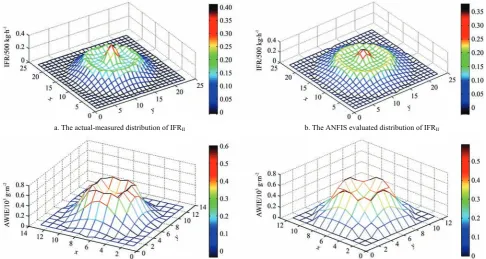
Losses (TL, %), and Infiltration Depth of soil ground (IDS, mm/h). Since the circular sprinkling radius of sprinkler nozzle is prearranged as 1.5 m, several interval distances of 0.6 m, 0.8 m, 1.0 m, 1.2 m, 1.5 m, 1.7 m, and 2.0 m are tested by sequence, in the interests of obtaining an optimal sprinkling uniformity to ensure the improved infiltration effectiveness, as Figure 6 gives the exampled planar distribution of sprinkler irrigation effectiveness level for reference.
5 Result and analysis
The results of sprinkler irrigation tests and ANFIS computations deliberately cover almost the entire value range of effectiveness indexes[44-47], the improved ANFIS we proposed in
this research would perform even better with fewer experiment turns. The versatility of ANFIS could be acknowledged easily when the effectiveness index evaluation is applied to study the correlative influences of inputs on outputs. For this aim, the evaluation of SIE indexes using ANFIS is regarded as a mathematical function of flow properties and orthogonal experiment employed by irrigation system, and the detailed process of ANFIS establishment can be learned from Liang et al.[43,48-51]
Here 25% of experimental cases are sampled out for instructive training, by which 50 turns are focused for network training and other cases for testing. It should be noted that each case is repeated for 100 trials to reduce any signal disturbance, and the resultant values of effectiveness indexes, including IFR, AWIE, TL, IDS, and Sl, should be averaged by these trials. Based on the
specialties of ANFIS in the evaluation process for irrigation effectiveness Table 4 proposes the information summary of network setting, Tables 5 and 6 respectively focuses on the partitioned levels of input parameters (flow properties including Rms, Ti, Tc, Te, and Rs), and output parameters (SIE indexes
including IFR, AWIE, TL, IDS, and Sl) for coding identification
and fuzzy reasoning. Combined with actual experimental processes, Table 7 describes the ANFIS logic rules being used, and Table 8 illustrates some exampled test conditions and evaluated irrigation effectiveness indexes on different soil layers, it could be observed that the increased flow RMS velocity would be accompanied by the precision decrease of SIE evaluation and the stability weakening of soil water seepage, due to a high probability of flow chaotic emerges in the diffusion of sprinkling water. On the other side, turbulence intensity and kinetic energy contribute greatly to the dynamic equilibrium of infiltration effectiveness indexes and saturated water content, thanks to the uniformed distributionoffluidviscosityandsoil water storage. Experimental
Table 4 Information summary of ANFIS setting
ANFIS settings Numbers and values
Nodes 66844
Linear weight values 44568
Nonlinear weight values 32584
Inputting parameters 446
Training data pairs 384
Checking data pairs 584
Fuzzy rules 10000
Training epochs 2400
Membership function Triangular-shape
verification also indicates that together with higher flow entropy, IFR, AWIE, and IDS slightly increase in an obviously tendency to over irrigation or infield infiltration variability. It can also be learned that there exists a stepping increase of AWIE and TL, in accordance with the increment of Reynolds shear stress for all the experimental conditions involved.
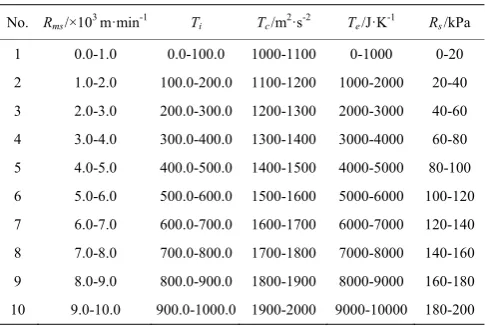
Table 5 Partitioned levels of input parameters (flow properties) and coding identification for ANFIS
No. Rms/×103 m·min-1 Ti Tc/m2·s-2 Te/J·K-1 Rs/kPa
1 0.0-1.0 0.0-100.0 1000-1100 0-1000 0-20 2 1.0-2.0 100.0-200.0 1100-1200 1000-2000 20-40 3 2.0-3.0 200.0-300.0 1200-1300 2000-3000 40-60 4 3.0-4.0 300.0-400.0 1300-1400 3000-4000 60-80 5 4.0-5.0 400.0-500.0 1400-1500 4000-5000 80-100 6 5.0-6.0 500.0-600.0 1500-1600 5000-6000 100-120 7 6.0-7.0 600.0-700.0 1600-1700 6000-7000 120-140 8 7.0-8.0 700.0-800.0 1700-1800 7000-8000 140-160 9 8.0-9.0 800.0-900.0 1800-1900 8000-9000 160-180 10 9.0-10.0 900.0-1000.0 1900-2000 9000-10000 180-200 Table 6 Partitioned levels of output parameters (SIE indexes)
and coding identification for ANFIS
No. Sl IFR/kg·h-1 AWIE/g·m-2 TL/% IDS/mm·h-1
1 0.00-1.00 1000.0-1050.0 200.0-280.0 0.00-1.00 20.0-23.0 2 1.00-2.00 1050.0-1100.0 280.0-360.0 1.00-2.00 23.0-26.0 3 2.00-3.00 1100.0-1150.0 360.0-440.0 2.00-3.00 26.0-29.0 4 3.00-4.00 1150.0-1200.0 440.0-520.0 3.00-4.00 29.0-32.0 5 4.00-5.00 1200.0-1250.0 520.0-600.0 4.00-5.00 32.0-35.0 6 5.00-6.00 1250.0-1300.0 600.0-680.0 5.00-6.00 35.0-38.0 7 6.00-7.00 1300.0-1350.0 680.0-760.0 6.00-7.00 38.0-41.0 8 7.00-8.00 1350.0-1400.0 760.0-840.0 7.00-8.00 41.0-44.0 9 8.00-9.00 1400.0-1450.0 840.0-920.0 8.00-9.00 44.0-47.0 10 9.00-10.00 1450.0-1500.0 920.0-1000.0 9.00-10.00 47.0-50.0 Table 7 Description of the ANFIS logic rules being used
No
Inputs Outputs
Rms Ti Tc Te Rs IFR AWIE TL IDS Sl
1 1 1 1 1 1 5 2 3 6 5 2 1 1 2 1 3 4 5 3 4 8
3 1 2 3 1 5 2 8 1 10 2
4 1 2 4 2 9 2 9 4 5 5 5 2 3 5 2 10 4 5 5 2 3 6 2 3 6 2 2 5 4 4 7 10 7 2 4 7 3 7 6 1 7 8 4 8 2 4 8 3 8 4 7 5 2 7 9 3 5 9 3 6 3 5 2 5 5
10 3 5 10 4 4 10 6 1 4 6
11 3 6 1 4 2 8 3 9 6 2
12 3 6 2 4 5 7 4 4 2 2
13 4 7 3 5 7 6 5 3 4 7
14 4 7 4 5 1 4 2 2 4 8
15 4 8 5 5 3 3 8 5 5 5
… …… ...
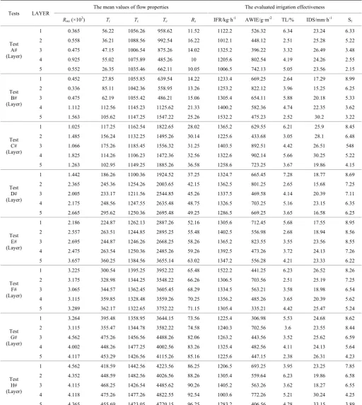
Table 8 Exampled test conditions and evaluated irrigation effectiveness values using ANFIS
Tests LAYER
The mean values of flow properties The evaluated irrigation effectiveness
Rms (×103) Ti Tc Te Rs IFR/kg·h-1 AWIE/g·m-2 TL/% IDS/mm·h-1 Sl
Test A# (Layer)
1 0.365 56.22 1056.26 958.62 11.52 1122.2 526.32 6.34 23.24 6.33
2 0.558 36.21 1088.56 992.54 16.22 1012.1 448.12 2.51 25.28 5.22
3 0.475 47.15 1006.54 875.26 14.02 1325.2 396.22 3.32 26.49 3.48
4 0.925 55.02 1075.89 485.26 10 1205.6 802.54 4.19 24.26 2.55
5 0.552 26.35 1035.46 662.11 10.05 1006.5 742.13 5.05 23.56 2.15
Test B# (Layer)
1 0.452 27.85 1055.85 639.54 14.22 1233.4 669.25 2.64 17.29 8.99
2 0.336 85.11 1042.36 558.95 13.26 1253.2 822.12 3.96 15.25 6.25
3 0.475 62.19 1055.42 486.21 15.06 1305.4 654.11 5.88 20.18 5.33
4 1.112 112.56 1145.23 1125.62 21.33 1400.2 582.36 4.74 22.35 3.62
5 1.563 105.62 1147.25 1547.22 25.26 1532.2 475.23 2.52 30.2 3.22
Test C# (Layer)
1 1.025 117.25 1162.54 1822.65 28.02 1365.2 629.55 6.21 25.9 8.45
2 1.485 156.24 1132.25 1495.26 30.14 1225.6 433.68 3.05 28.1 6.48
3 1.066 175.26 1185.45 1556.32 31.25 1403.5 892.51 4.42 26.51 548
4 1.825 114.26 1106.23 1472.36 32.56 1322.6 902.14 5.66 30.25 5.22
5 1.263 102.95 1149.25 1885.26 36.58 1258.6 723.25 3.67 19.86 4.15
Test D# (Layer)
1 1.442 186.26 1100.36 1924.52 37.25 1324.7 665.45 7.28 18.77 8.69
2 2.365 245.36 1254.26 2003.65 42.15 1362.5 801.25 2.65 15.68 7.25
3 2.005 233.17 1211.56 2544.85 45.26 1337.5 469.58 4.14 20.39 7.11
4 2.175 248.56 1247.55 2635.48 48.75 1326.5 703.25 5.16 23.15 6.35
5 2.665 295.62 1250.36 2695.48 49.25 1286.5 669.25 3.65 16.58 6.25
Test E# (Layer)
1 2.186 224.87 1262.13 2887.26 52.16 1305.6 712.45 5.68 17.55 8.95
2 2.557 263.51 1244.85 2895.25 55.48 1402.5 556.98 2.68 18.94 8.56
3 2.695 244.87 1246.26 2668.25 58.26 1365.2 823.55 3.55 23.56 8.55
4 2.475 263.54 1250.36 2485.26 59.26 1392.5 473.26 3.72 24.13 7.26
5 3.657 360.25 1384.56 3655.14 63.02 1347.2 556.28 4.21 23.33 6.22
Test F# (Layer)
1 3.225 300.54 1395.25 3952.22 65.48 1522.2 441.25 6.23 26.52 8.26
2 3.175 328.98 1344.25 3548.22 66.26 1306.5 703.56 2.51 25.19 7.25
3 3.065 344.57 1362.45 3605.45 68.29 1334.5 563.21 3.58 18.98 6.54
4 3.115 359.85 1328.48 3559.26 70.25 1356.2 485.26 3.65 20.39 5.62
5 3.289 362.17 1322.65 3752.22 71.15 1305.4 335.21 4.42 25.47 5.24
Test G# (Layer)
1 3.264 395.48 1358.95 3644.15 73.56 1225.4 306.98 5.53 24.68 8.62
2 3.115 355.47 1344.78 3582.22 74.58 1240.3 702.56 3.6 23.55 8.44
3 4.562 475.26 1456.56 4488.26 82.06 1263.2 443.56 3.52 25.62 6.59
4 4.002 448.26 1477.25 4002.56 83.26 1325.4 482.56 4.11 24.13 5.64
5 4.117 453.29 1426.56 4115.26 85.16 1225.6 447.15 2.38 26.31 4.23
Test H# (Layer)
1 4.562 418.59 1442.56 4223.56 86.25 1206.5 693.25 3.95 23.25 7.85
2 4.352 448.59 1482.56 4026.56 88.26 1305.4 559.64 6.23 19.86 6.58
3 4.115 468.25 1426.54 4485.62 90.26 1405.2 563.26 3.62 18.27 6.55
4 4.118 475.26 1477.26 4822.55 92.54 1003.6 772.26 5.21 30.24 4.25
5 4.365 455.69 1423.05 4720.15 96.25 1283.2 406.56 4.28 33.15 3.89
Note: Depth of layer 1: 0-100 cm; layer 2: 100-200 cm; layer 3: 200-300 cm; layer 4: 300-400 cm; layer 5: 400-500 cm. Figure 7 demonstrates the mean value comparisons of flow
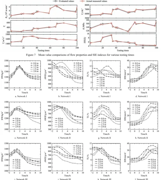
properties and SIE indexes for various testing times, a high agreement between the evaluated and actual measured SIE indexes could be identified easily. Based on these computations Figure 8 further explores the measured SIE indexes of typical irrigation networks with respect to different space intervals between sprinkler nozzles for various testing times and irrigation turn duration, as labeled from (a) to (t), which show that the actual measured SIE indexes, could be improved greatly to an ideal state of distributive equilibrium. As all these figures describe the result quantification
of cumulative moisture infiltration and the influence evaluations of irrigation effectiveness, the high consistency between them could be valued and referenced since which confirms the applicability and accuracy of this research.
dry one instead, so the evaporation process and TL could be accelerated remarkably. Air temperature frequently plays a remarkable influence on the moisture evaporation and TL in practice, a higher environmental temperature often accompanied by a higher evaporation and loss amount of water moisture. Besides, the amount of water evaporation keeps a positive correlation with solar radiation and soil-water content, but negative with the relative humidity in air ambience. During the given irrigation period everyday, the soil-water content or infiltration depth increases in the initial stage, then demonstrates a decreasing tendency
subsequently. However, the water evaporation or TL in soil ground decreases at the very first, then the consumption of transpiration increases greatly after 4 hours of sprinkler irrigation. From these observed phenomenons we can see that the moisture evaporation amount shows a strong correlation with some key influential factors ranked in descending order as: soil-water content, solar radiation, air relative humidity, wind speed, and air temperature, which could also be confirmed from the perspective of water use efficiency, soil evaporation, surface runoff and drainage, and ground circulation efficiency, etc[44-46].
Figure 7 Mean value comparisons of flow properties and SIE indexes for various testing times
a. Network I b. Network I c. Network I d. Network I
e. Network II f. Network II g. Network II h. Network II
m. Network IV n. Network IV o. Network IV p. Network IV
q. Network V r. Network V s. Network V t. Network V
Figure 8 Measured SIE indexes of various networks with respect to different space intervals between sprinkler nozzles To compare the evaluated SIE indexes with actual-measured
ones for proving their accuracy and reliability, a series of effective benchmark coefficients should be provided. In this research, using the AWIE of irrigation network III (to be labeled as AWIEIII)
as an example, its average relative percent error (APE) be defined as:
, ,
1 ,
1 ( ) ( )
100 ;
( )
n
III act i III eva i i i
i III act i
AWIE AWIE
APE E E
n = AWIE
⎡ − ⎤
= × = ⎢ ⎥
⎣ ⎦
∑
(11)The Absolute Average Relative Percent Error (AAPE) of AWIEIII is[51-53]:
The Absolute Average Relative Percent Error (AAPE) of AWIEIII is[51-53]:
, ,
1 ,
1 ( ) ( )
100 ;
( )
n
III act i III eva i i i
i III act i
AWIE AWIE
AAPE E E
n = AWIE
⎡ − ⎤
= × = ⎢ ⎥
⎣ ⎦
∑
(12)The Root Mean Square Error (RMSE) of AWIEIII is:
2 , , 1 1 ; ( ) ( ) n
i i III act i III eva i
i
RMSE e e AWIE AWIE
n =
=
∑
= − (13)The correlation coefficient (R) of AWIEIII can be defined as:
, 1 , 2 , 1 2 , 1 ( ) ( ) ( ) ( ) ( ) ( ) ( ) ( )
III act i III act n
i
III eva i III eva
n
III act i III act i
n
III eva i III eva i AWIE AWIE AWIE AWIE R AWIE AWIE AWIE AWIE = = = ⎛⎡⎣ − ⎤⎦⎞ ⎜ ⎟ ⎜⎡ ⎤⎟ ⎜⎣ − ⎦⎟ ⎝ ⎠ = ⎛ ⎡ − ⎤ ⎞ ⎜ ⎣ ⎦ ⎟ ⎜ ⎟ ⎜ ⎡ − ⎤ ⎟ ⎜ ⎣ ⎦ ⎟ ⎝ ⎠
∑
∑
∑
(14)where, (AWIEIII)act,i and (AWIEIII)eva,i stand for the ith measured and evaluated values of AWIEIII respectively; (AWIEIII act) and
(AWIEIII eva) denote their averaged values accordingly, and n denotes the number of irrigation tests. Then the Overall Relative Performance Factor (ORPF) of AWIEIII can be obtained as[52-54]:
min min
max min max min
(1 )
APE APE RMSE RMSE
ORFP R
APE APE RMSE RMSE
− −
= + + −
− −
(15)
After the effectiveness comparisons and influence analysis of Rms, Ti, Tc, Te, Rs, and Sl were completed, the ANFIS evaluations for flow properties and SIE compared with the measured ones are illustrated and discussed in Figure 9a-9f, as two solid lines in these figures identify the error range of ±10% for different SIE indexes[55,56]. For example, the ANFIS evaluation of Rms presents
APE of 2.056, AAPE of 2.335, RMSE of 0.417, R of 0.58, ORPF of 0.66; Evaluation of Ti presents APE of 4.227, AAPE of 3.621, RMSE of 0.825, R of 0.66, ORPF of 1.71; Evaluation of Tc presents APE of 4.005, AAPE of 2.331, RMSE of 0.824, R of 0.66, ORPF of 0.71; Evaluation of Te presents APE of 3.339, AAPE of 3.627, RMSE of 0.582, R of 0.41, ORPF of 1.66; Evaluation of Rs presents APE of 4.665, AAPE of 3.285, RMSE of 0.812, R of 0.26, ORPF of 1.74; and Evaluation of Sl presents APE of 5.227, AAPE
of 6.251, RMSE of 0.613, R of 0.47, ORPF of 1.58, ...etc. As Figures 10a-10h illustrate the distributive comparisons between the actual-measured and ANFIS-evaluated SIE indexes on a given irrigated area when different irrigation network being applied, as IFRII, AWIEIII, TLIV, and IDSV are enumerated sequentially as
representative examples, a high consistence between them can be learned, thus the computational precision of ANFIS evaluation can be ensured and a remarkable promotion in moisture infiltration equilibrium can be achieved. ANFIS also yields accurate influence mechanism and reliable quantitative evaluations for them, realizes an accurately demonstration of flow properties and returns effective theoretical basis to instruct a higher water circulation efficiency.
Based on these definitions and systematic computations the benchmark coefficient comparisons of SIE indexes could be shown by Table 9. To analyze their quantitative influences Figure 11 gives us a clear evaluative picture of them on given irrigated areas when different irrigation networks being applied, with its five axles stand for IFR, IDS, TL, Sl and AWIE respectively. We can see
a. APE=2.056; AAPE=2.335; RMSE=0.417; R=0.58; ORPF=0.66 b. APE=4.227; AAPE=3.621; RMSE=0.825; R=0.66; ORPF=1.71
c. APE=4.005; AAPE=2.331; RMSE=0.824; R=0.66; ORPF=0.71 d. APE=3.339;AAPE=3.627; RMSE=0.582; R=0.41; ORPF=1.66
e. APE=4.665; AAPE=3.285; RMSE=0.812;R=0.26; ORPF=1.74 f. APE=5.227; AAPE=6.251;RMSE=0.613; R=0.47; ORPF=1.58 Figure 9 ANFIS evaluations for flow properties and SIE compared with the measured ones
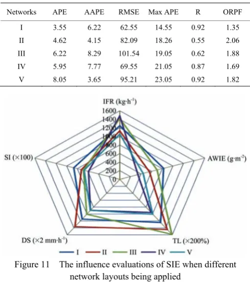
a. The actual-measured distribution of IFRII b. The ANFIS evaluated distribution of IFRII
e. The actual-measured distribution of TLIV f. The ANFIS evaluated distribution of TLIV
g. The actual-measured distribution of IDSV h. The ANFIS evaluated distribution of IDSV
Figure 10 The distributive comparisons between the actual-measured and ANFIS-evaluated SIE indexes on given irrigated areas when different irrigation network being applied
Table 9 The benchmark coefficient comparisons of SIE indexes between different network layouts
Networks APE AAPE RMSE Max APE R ORPF
I 3.55 6.22 62.55 14.55 0.92 1.35
II 4.62 4.15 82.09 18.26 0.55 2.06
III 6.22 8.29 101.54 19.05 0.62 1.88
IV 5.95 7.77 69.55 21.05 0.87 1.69
V 8.05 3.65 95.21 23.05 0.92 1.82
Figure 11 The influence evaluations of SIE when different network layouts being applied
On the other side, the statistic analysis of SIE(Sl) when
different irrigation networks are employed can also be learned from Figure 12, with its six axles stand for the APE, AAPE, RMSE, Max APE, R and ORPF of SIE respectively, simultaneously the accuracy levels of evaluative computation are highlighted by different colored hexagons. The one with a minimum area of enclosed hexagon frame suggests the most comprehensive working versatility and highest computational precision of influence analysis. For instance, the high convergence in APE emerges as network V is tested, which is suitable to control the amount of
sprinkling water or the consumption of deep percolation; network III ensures an excellent evaluation of SIE in AAPE and RMSE, for which provides an accurate effectiveness calibration of infiltration depth and water distribution efficiency, and keeps high credibility in the conditions of evaporation losses and non-productive run-off flows; network IV presents a satisfactory result in Max APE and shows a more-precisely evaluation result of SIE when transpiration losses or soil water seepage are concerned about. Network V deserves high attention in the benchmark coefficient of R and simultaneously focuses on the average irrigation efficiency, soil water redistribution, and moisture diffusivity as well; an excellent result could be recognized in ORPF when network II is tested, describing the fact that it proposes a robust evaluation of infiltration flow rate and transpiration losses for actual irrigation experiments[57-60].
In this research SPSS 19.0 is used for the statistical analysis and significant difference testing (Duncan method, α=0.05). As an influence illustration of sprinkler irrigation effectiveness on planting yields and water usage efficiency, Table 10 gives us a statistical schematic concerning with the remarkable productivity and quality developments during the whole experimental period, in such subjects as the planting yield, total amount of water consumption, irrigation quota, average efficiency of water usage, and the average efficiency of irrigation water, based on the influence analysis of sprinkler irrigation effectiveness achieved and the advantages of ANFIS evaluation confirmed. This table demonstrates that network III and IV show relatively lower water consumption than alternative does, especially an obviously decreased water consumption by 25.0%-25.5% in initial growth stage but steady in the following stages could be found, thus a more effective IFR and AWIE would be expected, which prevent the
moisture evaporation, TL and Sl value from exceeding a reasonable limit; Network IV and V promote AWIE and IDS and are suitable to be used for the control of vapor pressure deficit, thus the excessive moisture loss caused by water percolation and surface evaporation can be reduced greatly; the observed water consumption of network II or IV is decreased by 12.8% or 12.1% respectively compared with that of network I, so that TL could be reduced by 18.4% than that of network V, and lowered by 17.2% when compared with that of network III. The moisture feed evaporators of network VI and V keep in a relatively low level thereafter the utilization factor of sprinkling water and soil moisture for vegetation planting would be improved greatly. Furthermore, the water usage efficiency of network I or V can reach higher than that of network II and IV by 10.0%-17.3%, at the same time the infiltration effectiveness could be increased by 14.5%-32.7%, too.
Table 10 Influences of sprinkler irrigation effectiveness on planting yields and water usage efficiency
Network Planting yield /kg·hm-2
Total amount of water consumption/m3·hm-2
Irrigation quota /m3·hm-2
Average Efficiency of water usage/kg·m-3
Average Efficiency of irrigation water/kg·m-3
I 5635.41 3022.56 2844.51 5024.22 5647.25
II 6255.71 2875.15 2516.23 6244.25 6844.25
III 8922.15 4033.65 3477.56 7023.55 7511.24
IV 4822.65 2955.26 2670.25 4822.15 5348.25
V 7033.25 3466.21 3022.45 4617.22 4936.51
In addition, it is learned that when network I is employed, the water content monitored at the soil depth from 0 to 500 mm (with the same as follows) would change obviously from 19.7%-28.6%; By contrast, the water content and soil water seepage could be kept in a relatively steady state when network II is employed; the circulation efficiency of groundwater first decreases slowly and then increases subsequently when the working characteristics of network III are demonstrated; the soil water storage changed slightly between 20.8% and 21.3% when network IV is tested, which proves its distinctive capability of irrigation process stabilization in the subjects of water distributive efficiency and soil moisture uniformity. Finally, network V ensures a smooth irrigation performance in the moisture content and hydraulic conductivity from 21.4% to 26.7%, either.
Since the innovative ANFIS system and SIE indexes proposed in this investigation can be used as appropriate tools to quantify the complicated correlations between sprinkler irrigation and moisture infiltration, this work makes the following contributions for precision agriculture: (1) Objective of this research is implementing a novel influence analysis of sprinkler irrigation effectiveness (SIE) using ANFIS to improve actual irrigation quality; (2) A set of calibration indexes quantifying SIE are established and introduced to investigate its constructive influence mechanism; (3) ANFIS is designed and employed to assess SIE indexes and evaluate their far-reaching influences on the moisture infiltration balanced; (4) This study tries to make an integrated investigation of quantitative comparison and instructive influence analysis of SIE in different experimental conditions, thereafter the higher infiltration efficiency and better-balanced water distribution in soil field could be prompted.
6 Conclusions
This paper sought to achieve a detailed influence analysis of sprinkler irrigation effectiveness using ANFIS. The proposed calibration indexes of irrigation effectiveness assessing the
infiltration equilibrium of sprinkling water, and the comprehensive influence mechanism analyzed by ANFIS, are the main focuses of this investigation. Through measuring and collecting on-the-spot soil infiltration information with the application of tensionmeter in different field conditions, this research proposes an integrated set of SIE indexes, including IFR, AWIE, TL, and IDS, and then uses ANFIS to quantify their complicated interaction mechanism, on this basis the advantages and superiorities of this research aim at facilitating moisture infiltration efficiency could be verified in planting cultivation. This influence analysis provides novel instructions and precise benchmarks for the working assessment of sprinkler irrigation, and introduces new theoretical basis and far-reaching technical supports for the applicable irrigation qualification and the water balancing of agro-ecosystem afterwards.
Acknowledgements
thank the editors for their hard work and the referees for their kindly comments and valuable suggestions to improve this paper.
[References]
[1] Li M, Fu Q, Singh V P, Liu D. An interval multi-objective programming model for irrigation water allocation under uncertainty. Agric.Water Manag., 2018; 196(31): 24–36.
[2] Dai Z, Li Y. A multistage irrigation water allocation model for agricultural land-use planning under uncertainty. Agric.Water Manag., 2013; 129(6): 69–79.
[3] Guo P, Chen X, Li M, Li J. Fuzzy chance-constrained linear fractional programming approach for optimal water allocation. Stoch. Env. Res. Risk A., 2014; 28(6): 1601–1612.
[4] Li M, Guo P. A multi-objective optimal allocation model for irrigation water resources under multiple uncertainties. Appl. Math. Model., 2014; 38 (19-20): 4897–4911.
[5] Liu X, Liang Z, Wen G, Yuan X. Waterjet machining and research developments: a review. Int. J. Adv. Manuf. Technol., 2018; 102(5): 1257–1335.
[6] Ward F A, Crawford T L. Economic performance of irrigation capacity development to adapt to climate in the American Southwest. J. Hydrol., 2016; 540(9): 757–773.
[7] Habteyes B G, El-bardisy H A, Amer S A, Schneider V R, Ward F A. Mutually beneficial and sustainable management of Ethiopian and Egyptian dams in the Nile Basin. J. Hydrol., 2015; 529(10): 1235–1246. [8] Hellín H N, Rincon J M, Miguel R D, Valles F S, Sánchez R T. A
decision support system for managing irrigation in agriculture. Comput. Electron. Agr., 2016; 124(c): 121–131
[9] Opan M. Irrigation-energy management using a DPSA-based optimization model in the Ceyhan basin of Turkey. J. Hydrol., 2010; 385(1): 353–360.
[10] Liang Z, Liu X. Fuzzy performance between surface fitting and energy distribution in turbulence runner. Sci. World J., 2012; 25(10): 408949 [11] Robles J M, Botía P, Pérez J G. Subsurface drip irrigation affects trunk
diameter fluctuations inlemon trees, in comparison with surface drip irrigation. Agric.Water Manag., 2016; 165(2): 11–21
[12] Wakchaure G C, Minhas P S, Ratnakumar P, Choudhary R L. Optimising supplemental irrigation for wheat and the impact of plant bio-regulators in a semi-arid region of Deccan Plateau in India. Agric.Water Manag., 2016; 172(2016): 9–17
[13] Reca J, Torrente C, Luque L, Martinez J. Feasibility analysis of a stand alone direct pumping photo voltaic system for irrigation in Mediterranean greenhouses. Renew. Energy, 2016; 85(1): 1143–1154
[14] Crespo O, Bergez J E, Garcia F. Multiobjective optimization subject to uncertainty: Application to irrigation strategy management. Comput. Electron. Agr, 2010; 74(1): 145–154
[15] Barradas J M, Matula S, Dolezal F. A decision support system-fertigation simulator (DSS-FS) for design and optimization of sprinkler and drip irrigation systems. Comput. Electron. Agr, 2012; 86(6): 111–119 [16] Jiang L, Shang S, Yang Y, Guan H. Mapping inter annual variability of
maize cover in a large irrigation district using a vegetation index-phenological index classifier. Comput. Electron. Agr, 2016; 123(4): 351–361.
[17] Nieto P, Gonzalo E G, Arbat G, Ros M D, Cartagena F R, Bargués J P. A new evaluateive model for the filtered volume and outlet parameters in micro-irrigation sand filters fed with effluents using the hybrid PSO-SVM- based approach. Comput. Electron. Agr, 2016; 125(7): 74–80.
[18] Nasiakou A, Vavalis M, Zimeris D. Smart energy for smart irrigation. Comput. Electron. Agr, 2016; 129(11): 74–83.
[19] Linker R, Sylaios G. Efficient model-based sub-optimal irrigation scheduling using imperfect weather forecasts. Comput. Electron. Agr., 2016; 130(11): 118–127
[20] Campana P E, Li H, Zhang J, Zhang R, Liu J, Yan J. Economic optimization of photovoltaic water pumping systems for irrigation. Energy Convers. Manag., 2015; 95(5): 32–41.
[21] Kovacs K F, Mancini M, West G. Landscape irrigation management for maintaining an aquifer and economic returns. J. Environ. Manage., 2015; 160(7): 271–282.
[22] Liang Z, Liu X, Zhou J, Liao S. Video tracking for high- similarity drug tablets based on reflective energy intensity matrix and fuzzy recognition system. Proc IMechE Part H: J Eng. Med., 2016; 230(3): 211–229. [23] Evan M, Ru W, Xia X. Energy-water optimization model incorporating
rooftop water harvesting for lawn irrigation. Appl. Energy, 2015; 160(12): 521–531.
[24] Campana P E, Leduc S, Kim M, Olsson A, Zhang J, Liu J, et al. Suitable and optimal locations for implementing photovoltaic water pumping systems for grassland irrigation in China. Appl. Energy, 2017; 185(1):1879–1889.
[25] Garga N K, Dadhich S M. Integrated non-linear model for optimal cropping pattern and irrigation scheduling under deficit irrigation. Agric.Water Manag., 2014; 140(1): 1–13.
[26] Koech R K, Smith R J, Gillies M H. Evaluating the performance of a real-time optimisation system for furrow irrigation. Agric.Water Manag., 2014; 142(142):77–87.
[27] Hellín H N, Sánchez R T, Valles F S, Pérez C A, Riquelme J A, Miguel R D. A wireless sensors architecture for efficient irrigation water management. Agric.Water Manag., 2015; 151(3): 64–74.
[28] Esfahani L H, Rua A T, McKee M. Assessment of optimal irrigation water allocation for pressurized irrigation system using water balance approach, learning machines,and remotely sensed data. Agric.Water Manag., 2015; 153(2): 42–50.
[29] Yang G, Guo P, Huo L, Ren C. Optimization of the irrigation water resources for Shijin irrigation district in north China. Agric. Water Manag., 2015; 158(8): 82–98.
[30] Pascual M, Villar J M, Rufat J. Water use efficiency in peach trees over a four-years experiment on the effects of irrigation and nitrogen application. Agric.Water Manag., 2016; 164(1): 253–266.
[31] Domingo R J, Arbonés X, Pascual A, Villar M. Interaction between water and nitrogen management in peaches for processing. Irrig. Sci., 2011; 29(4): 321–329.
[32] Skewes P V, Cox M A, Mahadevan J W. Modelling the impact of pulsing of drip irrigation on the water and salinity dynamics in soil in relation to water uptake by an almond tree. WIT Trans. Ecol Environ., 2012; 168(19): 101–113.
[33] Kranz W L, Evans R G, Lamm R G, Shaughnessy S A, Peters R T. A review of mechanical move sprinkler irrigation control and automation technologies. Appl. Eng. Agric. ASABE, 2012; 28 (3): 389–397. [34] García F, Montesinos I, Poyato P C, Díaz E R. Energy cost optimization
in pressurized irrigation networks. Irrig. Sci., 2016; 34(1): 1–13. [35] Alison M, Nigel C H, Steven R. Simulation of irrigation control
strategies for cotton using model evaluateive control within the VARI wise simulation framework. Comput. Electron. Agric., 2014; 101(5): 135–147. [36] Sayyadi H, Sadraddini A A, Zadeh D F, Montero J. Artificial neural
networks for simulating wind effects on sprinkler distribution patterns. Span. J. Agric. Res., 2012; 10(4): 1143–1154.
[37] Liang Z W, Tan S S, Liao S P, Liu X C. Component parameter optimization of strengthen waterjet grinding slurry with the improved ANFIS. Int. J. Adv. Manuf. Technol., 2017; 90(12): 831–855.
[38] Xue X Y, Tu K, Qin W C, Lan Y B, Zhang H H. Drift and deposition of ultra-low altitude and low volume application in paddy field. Int. J. Agric. & Biol. Eng., 2014; 7(4): 23–28.
[39] Zheng Y J, Yang S H, Zhao C J, Chen L P, Lan Y B, Tan Y. Modelling operation parameters of UAV on spray effects at different growth stages of corns. Int. J. Agric. & Biol. Eng., 2017; 10(3): 57–66.
[40] Liang Z, Liao S, Wen Y, Liu X. Working parameter optimization of strengthen waterjet grinding with the improved ANFIS. J. Intell. Manuf., 2016; 30(2): 833–854.
[41] Guo P, Wang X, Zhu H, Li M. Inexact fuzzy chance-constrained nonlinear programming approach for crop water allocation under sprinkling water variation and sustainable development. J. Water Resour. Plann. Manag., 2014; 140 (9): 5014003.
[42] Chen S D, Lan Y B, Li J Y, Zhou Z Y, Liu A M, Mao Y D. Effect of wind field below unmanned helicopter on droplet deposition distribution of aerial spraying. Int. J. Agric. & Biol. Eng., 2017; 10(3): 67–77.
[43] Liang Z, Liu X. Four-dimensional fuzzy relation investigation in turbulence kinetic energy distribution, surface cluster modeling, Arab. J. Sci. Eng. 2014; 39(1): 2339–2351.
[44] Tong F F, Guo P. Simulation and optimization for crop water allocation based on crop water production functions and climate factor under uncertainty. Appl. Math. Model., 2013; 37(14-15): 7708–7716
[45] Dukes M D. Water conservation potential of landscape irrigation smart controllers. Trans. ASABE, 2012; 55(2): 563–569.
index to incorporate the irrigation performance and reservoir operations: A case study in the Tarim river basin. Global Planet. Change, 2016; 143(8): 10–20.
[48] Maia R, Silv C, Costa E. Eco-efficiency assessment in the agricultural sector: the Monte Novo irrigation perimeter, Portugal. J. Clean. Prod., 2016; 138(12): 217–228.
[49] Vila M G, Fereres E. Combining the simulation crop model Aqua Crop with an economic model for the optimization of irrigation management at farm level. Europ. J. Agron., 2012; 36(1): 21–31.
[50] Hou C J, Tang Y, Luo S M, Lin J T, He Y, Zhuang J J, et al. Optimization of control parameters of droplet density in citrus trees using UAVs and the Taguchi method. Int J Agric & Biol Eng, 2019; 12(4): 1–9. [51] Liang Z, Shan S, Liu X, Wen Y. Fuzzy evaluation of AWJ flow
properties by using multi-phase flow models. Eng. Appl. Comp. Fluid, 2017; 11(1): 225–257.
[52] Cheviron B, Vervoort R W, Albasha R, Dairon R, L Priol C, Mailhol J C. A framework to use crop models for multi-objective constrained optimization of irrigation strategies. Environ. Modell. Softw., 2016; 86(c): 145–157.
[53] Izquiel A, Carrion P, Tarjuelo J M, Moreno M A. Optimal reservoir capacity for centre pivot irrigation water supply: Maize cultivation in Spain. Biosyst. Eng., 2015; 135(7): 61–72.
[54] Liang Z W, Liu X C, Ye B Y, Wang Y J. Performance investigation of fitting algorithms in surface micro- topography grinding processes based on multi- dimensional fuzzy relation set, Int. J. Adv. Manuf. Technol., 2013; 67(7): 2779–2798.
[55] Izquiel A, Ballesteros R, Tarjuelo J M, Moreno M A. Optimal reservoir sizing in on-demand irrigation networks: Application to a collective drip irrigation network in Spain. Biosyst. Eng., 2016; 147(5): 67–80. [56] Zhang P, Deng L, Lyu Q, He S L, Yi S L, Liu Y D, et al. Effects of citrus
tree-shape and spraying height of small unmanned aerial vehicle on droplet distribution. Int J Agric & Biol Eng, 2016; 9(4): 45–52.
[57] Liang Z W, Ye B Y. Three-dimensional fuzzy influence analysis of fitting algorithms on integrated chip topographic modeling. J. Mech. Sci. Technol., 2012; 26(10): 3177–3191.
[58] Bekchanov M, Ringler C, Bhaduri A, Jeulan M. Optimizing irrigation efficiency improvements in the Aral Sea Basin. Water. Resour. Res., 2016; 13(1): 30–45.
[59] Tinoco V, Willems P, Wyseure G, Cisneros F. Evaluation of reservoir operation strategies for irrigation in the Macul Basin, Ecuador. J. Hydrol.: Regional Studies., 2016; 5(c): 213–225.