Study and comparison of various image edge detection techniques
used in quality inspection and evaluation of agricultural and
food products by computer vision
V G Narendra
,
K S Hareesh
(Department of Computer Science and Engineering, Manipal Institute of Technology,Manipal,Karnataka,India-576104)
Abstract:Edges characterize boundaries and are therefore a problem of fundamental importance in quality assessment of agricultural and food products. Since edge detection is in the forefront of computer vision system for detection of vegetables, fruits and food grains needs to quality inspection and evaluation, it is crucial to have a good understanding of edge detection algorithms. In this paper the comparative analysis of various image edge detection techniques is presented. The software is developed using MATLAB 7.6. It has been shown that the Canny’s edge detection algorithm performs better than all operators (i.e. LoG, Robert, Prewitt and Sobel ) under almost all scenarios.
Keywords:edge detection, noise, computer vision, agricultural and food products
DOI:10.3965/j.issn.1934-6344.2011.02.083-090
Citation:Narendra V G, Hareesh K S. Study and comparison of various image edge detection techniques used in quality inspection and evaluation of agricultural and food products by computer vision. Int J Agric & Biol Eng, 2011; 4(2): 83-90.
1
Introduction
Edge detection refers to the process of identifying and
locating sharp discontinuities in an image like vegetables,
fruits and food grains. The discontinuities are abrupt
changes in pixel intensity which characterize boundaries
of objects in an image. Classical methods of edge
detection involve convolving the image with an operator
(a 2-D filter), which is constructed to be sensitive to large
gradients in the image while returning values of zero in
uniform regions. This is an extremely large number of
edge detection operators available, each designed to be
sensitive to certain types of edges. Variables involved in
the selection of an edge detection operator include:
1) Edge orientation: The geometry of the operator
Received date:2010-08-09 Accepted date:2011-04-11
Corresponding author: K S Hareesh, Associate Professor, Department of Computer Science and Engineering, Manipal Institute of Technology, Manipal, Karnataka, India-576104. Email: [email protected]; hareesh. ks@manipal. edu.
determines a characteristic direction in which it is most
sensitive to edges. Operators can be optimized to look
for horizontal, vertical, or diagonal edges.
2) Noise environment: Edge detection is difficult in
noisy images, since both the noise and the edges contain
high-frequency content. Reducing the noise will result
in blurred and distorted edges. Operators used in noisy
images are typically larger in scope, so they can average
enough data to discount localized noisy pixels. This
results in less accurate localization of the detected edges.
3) Edge structure: Not all edges involve a step change
in intensity. Effects such as refraction or poor focus can
result in objects with boundaries defined by a gradual
change in intensity. The operator needs to be chosen to
be responsive to such a gradual change in those cases.
Newer wavelet-based techniques actually characterize the
nature of the transition for each edge in order to
distinguish, for example, edges associated with hair from
edges associated with a face.
However, the majority of different methods may be
grouped into two categories: Gradient and Laplacian[1-6]. The primary objective is first we analyzed the various
edge detection techniques (i.e. LoG, Robert, Prewitt,
Zero-cross, canny and Sobel) and shown the visual
comparisons of various edge detection techniques.
The visual comparison of the most commonly used
Gradient and Laplacian based edge detection techniques
was analyzed and performed. In Section 2 the problem
definition with the Gradient and Laplacian working
methods is presented. In Section 3 the various edge
detection techniques have been studied and analyzed. In
Section 4 the visual comparisons of various edge
detection techniques have been done by developing
software in MATLAB 7.6. Section 5 discusses the
advantages and disadvantages of various edge detection
techniques. Section 6 discusses the conclusions reached
by analysis and visual comparison of various edge
detection techniques developed using MATLAB 7.6.
2
Problem definition
There are problems of false edge detection, missing
true edges, producing thin or thick lines and problems due
to noise etc. We analyzed and performed the visual
comparison of the most commonly used Gradient and
Laplacian based edge detection techniques for problems
of inaccurate edge detection, missing true edges,
producing thin or thick lines and problems due to noise
etc. The software is developed using MATLAB 7.6.
The methods of most commonly used Gradient and
Laplacian based edge detection techniques are as follows.
2.1 Gradient
The gradient method detects the edges by looking for
the maximum and minimum in the first derivative of the
image.
2.2 Laplacian
The Laplacian method searches for zero crossings in
the second derivative of the image to find edges. An edge
has the one-dimensional shape of a ramp and calculating
the derivative of the image can highlight its location.
Suppose we have the following signal, with an edge shown
by the jump in intensity (Figure 1)[2,6].
Suppose we have the following signal, with an edge
shown by the jump in intensity (shown in Figure 1).
Figure 1 Following signal applied to the edge detector
If we take the gradient of this signal (which, in one
dimension, is just the first derivative with respect tot) we
get the following (shown in Figure 2).
Figure 2 Gradient first derivative signal
Clearly, the derivative shows (Figure 2) a maximum
located at the center of the edge in the original signal.
This method of locating an edge is characteristic of the
“gradient filter” family of edge detection filters and
includes the Sobel method. A pixel location is declared
an edge location if the value of the gradient exceeds some
threshold. As mentioned before, edges will have higher
pixel intensity values than those surrounding it. So once
a threshold is set, you can compare the gradient value to
the threshold value and detect an edge whenever the
threshold is exceeded[6,7].
Furthermore, when the first derivative is at a
maximum, the second derivative is zero. As a result,
another alternative to find the location of an edge is to
locate the zeros in the second derivative. This method is
known as the Laplacian and the second derivative of the
Figure 3 Gradient second derivative signal
3
Edge detection techniques
3.1 Sobel operator
The operator consists of a pair of 3×3 convolution
kernels as shown in Figure 4. One kernel is simple, the
other rotated by 90°.
a.Gx b.Gy
Figure 4 Masks used by Sobel operator
These kernels are designed to respond maximally to
edges running vertically and horizontally relative to the
pixel grid, one kernel for each of the two perpendicular
orientations. The kernels can be applied separately to
the input image, to produce separate measurements of the
gradient component in each orientation (call theseGxand
Gy). These can then be combined together to find the
absolute magnitude of the gradient at each point and the
orientation of that gradient[6,8]. The gradient magnitude is given by:
2 2
|G| Gx Gy (1)
Typically, an approximate magnitude is computed
using:
|G| |Gx||Gy| (2)
Which is much faster to compute.
The angle of orientation of the edge (relative to the
pixel grid) giving rise to the spatial gradient is given by:
arctan(Gy Gx/ )
(3)
3.2 Robert’s cross operator
The Roberts Cross operator performs a simple and
quick computing, 2-D spatial gradient measurement on an
image. Pixel values at each point in the output represent
the estimated absolute magnitude of the spatial gradient
of the input image at that point. The operator consists of
a pair of 2×2 convolution kernels as shown in Figure 5.
One kernel is simply the other rotated by 90°[6,9]. This is very similar to the Sobel operator.
a.Gx b.Gy
Figure 5 Masks used for Robert operator.
These kernels are designed to respond maximally to
edges running at 45°to the pixel grid, one kernel for each
of the two perpendicular orientations. The kernels can
be applied separately to the input image, to produce
separate measurements of the gradient component in each
orientation (call these Gx and Gy). These can then be
combined together to find the absolute magnitude of the
gradient at each point and the orientation of that gradient.
The gradient magnitude is given by Equation (1).
Although typically, an approximate magnitude is
computed using Equation (2), which is much faster to
compute.
The angle of orientation of the edge giving rise to the
spatial gradient (relative to the pixel grid orientation) is
given by
arctan(Gy Gx| ) 3 / 4
(4)
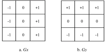
3.3 Prewitt’s
Prewitt operator[2]is similar to the Sobel operator and is used for detecting vertical and horizontal edges in
images.
a.Gx b.Gy
3.4 Laplacian of Gaussian
The Laplacian is a 2-D isotropic measure of the 2nd
spatial derivative of an image. The Laplacian of an
image highlights regions of rapid intensity change and is
therefore often used for edge detection. The Laplacian
is often applied to an image that has first been smoothed
with something approximating a Gaussian Smoothing
filter in order to reduce its sensitivity to noise. The
operator normally takes a single gray level image as input
and produces another gray level image as output. The
Laplacian L(x,y) of an image with pixel intensity values
I(x,y) is given by:
2 2
2 2
( , ) I I
L X Y
x y
(5)
Since the input image is represented as a set of
discrete pixels, we have to find a discrete convolution
kernel that can approximate the second derivatives in the
definition of the Laplacian[2]. Three commonly used
small kernels are shown in Figure 7.
Figure 7 Three commonly used discrete approximations to the Laplacian filter
Because these kernels are approximating a second
derivative measurement on the image, they are very
sensitive to noise. To counter this, the image is often
Gaussian Smoothed before applying the Laplacian filter.
This pre-processing step reduces the high frequency noise
components prior to the differentiation step.
In fact, since the convolution operation is associative,
we can convolve the Gaussian smoothing filter with the
Laplacian filter first of all, and then convolve this hybrid
filter with the image to achieve the required result.
Doing things this way has two advantages: Since both the
Gaussian and the Laplacian kernels are usually much
smaller than the image, this method usually requires far
fewer arithmetic operations.
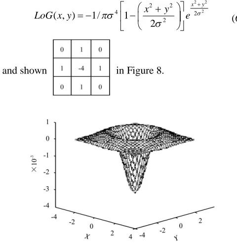
The LoG (‘Laplacian of Gaussian’)[10] kernel can be
pre-calculated in advance so only one convolution needs
to be performed at run-time on the image. The 2-D LoG
function[6,11]centered on zero and with Gaussian standard deviationσhas the form:
2 2 2
2 2
4 2
2
( , ) 1/ 1
2
x y
x y
LoG x y e
(6)
and shown in Figure 8.
Figure 8 2-D Laplacian of Gaussian (LoG) function. Thexandyaxes are marked in standard deviations (σ)
A discrete kernel that approximates this function (for
a Gaussianσ= 1.4) is shown in Figure 9.
Figure 9 Discrete approximation toLoGfunction with Gaussian = 1.4
Note that as the Gaussian is made increasingly narrow,
theLoGkernel becomes the same as the simple Laplacian
with a very narrow Gaussian (σ< 0.5 pixels) on a discrete
grid has no effect. Hence on a discrete grid, the simple
Laplacian can be seen as a limiting case of the LoG for
narrow Gaussians[6,12-14].
3.5 Canny edge detection algorithm
The Canny edge detection algorithm is known to
many as the optimal edge detector. Canny’s intentions
were to enhance the many edge detectors already out at
the time he started his work. He was very successful in
achieving his goal and his ideas and methods can be
found in his paper, “A Computational Approach to Edge
Detection”[6,15]. In his paper, he followed a list of
criteria to improve current methods of edge detection.
The first and most obvious is low error rate. It is
important that edges occurring in images should not be
missed and that there be no responses to non-edges. The
second criterion is that the edge points be well localized.
In other words, the distance between the edge pixels as
found by the detector and the actual edge is to be at a
minimum. A third criterion is to have only one response
to a single edge. This was implemented because the
first two were not substantial enough to completely
eliminate the possibility of multiple responses to an edge.
This is a multi-step edge detection procedure by
Canny[15]. The purpose of the following two methods is
to detect edges with noise suppressed at the same time.
1) Smooth the image with a Gaussian filter to reduce
noise and unwanted details and textures.
( , ) ( , ) ( , )
g m n G m n f m n (7)
Where,
(8)
Compute gradient of g(m ,n) by using any of the
gradient operators ( Sobel, Prewitt, etc) to get:
2 2
( , ) ( , ) ( , )
M m n g m m n g n m n (9)
and
(10)
2) ThresholdM:
( , ) ( , )
0
T
M m n M m n
ifM(m,n) >Totherwise 0 (11)
WhereT is so chosen that all edge elements are kept
while most of the noise is suppressed.
3) Suppress non-maxima pixels in the edges in MT
obtained above to thin the edge ridges (as the edges might
have been broadened in step 1). To do so, check to see
whether each non-zero MT (m, n) is greater than its two
neighbors along the gradient direction θ(m, n). If so,
keepMT(m,n) unchanged, otherwise, set it to 0.
4) Threshold the previous result by two different
thresholds T1 and T2 (where T1< T2) to obtain two
binary images T1 and T2. Note that compared toT1, T2
has less noise and fewer false edges but larger gaps
between edge segments.
5) Link edges segments in T2 to form continuous
edges. To do so, trace each segment inT2 to its end and
then search its neighbors inT1 to find any edge segment
in T1 to bridge the gap until reaching another edge
segment inT2.
4
Visual comparison of various edge detection
algorithms
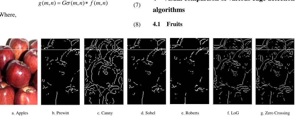
4.1 Fruits
a. Apples b. Prewitt c. Canny d. Sobel e. Roberts f. LoG g. Zero Crossing
4.2 Grains
a. Rice b. Prewitt c. Canny d. Sobel
e. Roberts f. LoG g. Zero Crossing
Figure 11 Canny is the best among results of fruit image edge detection
4.3 Bakery food product
a. Pizza b. Prewitt c. Canny d. Sobel
e. Roberts f. LoG g. Zero Crossing
Figure 12 Canny is the best among results of fruit image edge detection
Edge detection of all four types was performed
on above Figures 10a, 11a and 12a[16]. Canny yielded
the best results. This was expected as Canny edge
detection accounts for regions in an image. Canny
yields thin lines for its edges by using non-maximal
suppression. Canny also utilizes hysteresis with
thresholding.
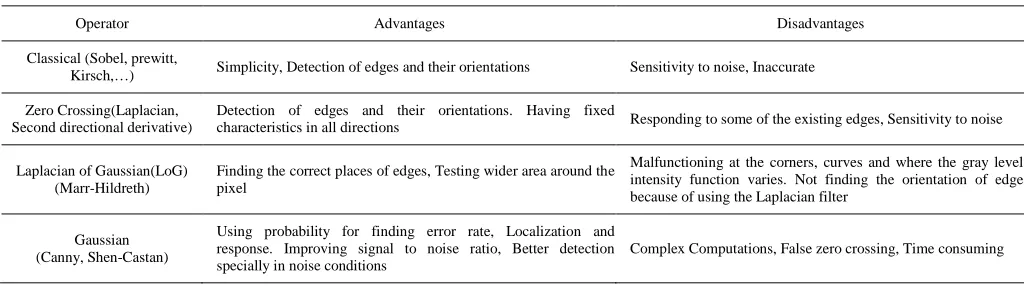
5 Advantages and disadvantages of edge detector
As edge detection is a fundamental step in computer
vision, it is necessary to point out the true edges to get the
best results from the matching process. That is why it is
important to choose edge detectors that fit best to the
application. In this respect, we first present some
advantages and disadvantages of edge detection
Table 1 Some advantages and disadvantages of edge detectors
Operator Advantages Disadvantages
Classical (Sobel, prewitt,
Kirsch,… ) Simplicity, Detection of edges and their orientations Sensitivity to noise, Inaccurate
Zero Crossing(Laplacian, Second directional derivative)
Detection of edges and their orientations. Having fixed
characteristics in all directions Responding to some of the existing edges, Sensitivity to noise
Laplacian of Gaussian(LoG) (Marr-Hildreth)
Finding the correct places of edges, Testing wider area around the pixel
Malfunctioning at the corners, curves and where the gray level intensity function varies. Not finding the orientation of edge because of using the Laplacian filter
Gaussian (Canny, Shen-Castan)
Using probability for finding error rate, Localization and response. Improving signal to noise ratio, Better detection specially in noise conditions
Complex Computations, False zero crossing, Time consuming
6
Conclusions
Since edge detection is the initial step in object
recognition, it is important to know the differences
between edge detection techniques. In this paper we
studied the most commonly used edge detection
techniques of Gradient-based and Laplacian based edge
detection. The software is developed using MATLAB
7.6.
Gradient-based algorithms such as the Prewitt filter
have a major drawback of being very sensitive to noise.
The size of the kernel filter and coefficients are fixed and
cannot be adapted to a given image. An adaptive
edge-detection algorithm is necessary to provide a robust
solution that is adaptable to the varying noise levels of
these images to help distinguish valid image contents
from visual artifacts introduced by noise.
The performance of the Canny algorithm depends
heavily on the adjustable parameters, σ, which is the
standard deviation for the Gaussian filter, and the
threshold values, ‘T1’and ‘T2’.σalso controls the size of
the Gaussian filter. The bigger the value for σ, the
larger the size of the Gaussian filter becomes. This
implies more blurring, necessary for noisy images, as
well as detecting larger edges. As expected, however,
the larger the scale of the Gaussian, the less accurate is
the localization of the edge. Smaller values ofσimply a
smaller Gaussian filter which limits the amount of
blurring, maintaining finer edges in the image. The user
can tailor the algorithm by adjusting these parameters to
adapt to different environments.
Canny’s edge detection algorithm is computationally
more expensive compared to Sobel, Prewitt and Robert’s
operator. However, the Canny’s edge detection
algorithm performs better than all these operators under
almost all scenarios. Evaluation of the images showed
that under noisy conditions, Canny, LoG, Sobel, Prewitt,
Roberts’s exhibit better performance, respectively.
Acknowledgements
The authors are greatly indebted to the Department of
Computer Science and Engineering, Manipal Institute of
Technology, Manipal University, Manipal for providing
excellent lab facilities that made this work possible.
[References]
[1] Argyle. E. Techniques for edge detection. In: Proceedings of IEEE, 1971; 59, 285–286.
[2] Gonzalez R C, Woods R E. Digital image processing. 2nd Ed. Prentice Hall, 2002.
[3] Heath M, Sarkar S, Sanocki T, Bowyer K W. Comparison of edge detectors: A methodology and initial study. Computer Vision and Image Understanding, 1998; 69(1): 38–54. [4] Shin M C, Goldgof D, Bowyer K W. Comparison of edge
detector performance through use in an object recognition task. Computer Vision and Image Understanding, 2001; 84(1): 160–178.
[5] Peli T, Malah D. A study of edge detection algorithms. Computer Graphics and Image Processing, 1982; 20: 1–21. [6] Maini R, Aggarwal H. Study and comparison of various
image edge detection techniques. International Journal of Image Processing (IJIP), 2009; 3(1).
[7] Bergholm F. Edge focusing. In: Proceedings of 8th International Conference on Pattern Recognition, Paris, France, 1986; pp. 597–600.
[9] Roberts L G. Machine perception of 3-D solids-series. Optical and Electro-Optical Information Processing. MIT Press, 1965.
[10] Torre V, Poggio T A. On edge detection. IEEE Trans. Pattern Anal. Machine Intell., 1986; 8(2): 187–163.
[11] Davies E R. Constraints on the design of template masks for edge detection. Pattern Recognition Lett., 1986; 4(2): 111-120.
[12] Frei W, Chen C C. Fast boundary detection: A generalization and a new algorithm. lEEE Trans. Comput., 1977; 26(10): 988–998.
[13] Grimson W E, Hildreth E C. Comments on digital step edges from zero crossings of second directional derivatives. IEEE Trans. Pattern Anal. Machine Intell, 1985; 7: 121–129. [14] Haralick R M. Digital step edges from zero crossing of the
second directional derivatives. IEEE Trans. Pattern Anal. Machine Intell, 1984; 6(1): 58–68.
[15] Canny J F. “A computational approach to edge detection”. IEEE Trans. Pattern Anal. Machine Intell. 1986; 8(6):
679–697.
[16] Kirsch R A. Computer determination of the constituent structure of biomedical images. Comput. Eiorned. Res, 1971; 4: 315–328.
[17] Hueckel M H. A local visual operator which recognizes edges and line. JACM. 1973; 20(4): 634–647.
[18] Yakimovsky Y. Boundary and object detection in real world images. JACM. 1976; 23(4): 598–619.
[19] Yuille A, Poggio T A. Scaling theorems for zero crossings. IEEE Trans. Pattern Anal. Machine Intell., 1986; 8(1): 187–163.
[20] Marr D, Hildreth E. Theory of edge detection. In: Proceedings of the Royal Society of London. Series B, Biological Sciences, 29th February, 1980; 207(1167): 187–217.