Road Segmentation with Neural Networks

Scholarly Horizons: University of Minnesota, Morris

Undergraduate Journal

Volume 5 | Issue 2

Article 5

June 2018

Road Segmentation with Neural Networks

Tsz Hong (Andy) Lau

University of Minnesota, Morris

Follow this and additional works at:

https://digitalcommons.morris.umn.edu/horizons

Part of the

Computer Sciences Commons

This Article is brought to you for free and open access by the Journals at University of Minnesota Morris Digital Well. It has been accepted for inclusion in Scholarly Horizons: University of Minnesota, Morris Undergraduate Journal by an authorized editor of University of Minnesota Morris Digital Well. For more information, please [email protected].

Recommended Citation

Lau, Tsz Hong (Andy) (2018) "Road Segmentation with Neural Networks,"Scholarly Horizons: University of Minnesota, Morris Undergraduate Journal: Vol. 5 : Iss. 2 , Article 5.

Cover Page Footnote

Road Segmentation with Neural Networks

Tsz Hong (Andy) Lau

Division of Science and Mathematics University of Minnesota, Morris Morris, Minnesota, USA 56267

[email protected]

ABSTRACT

Autonomous driving is the next biggest technological ad-vance in the automobile industry. However, the current tech-nology is still very much in its infancy. Networks of sensors such as cameras and LIDAR systems are used to record and measure the road condition. While neural networks are used to understand the road condition and make the correct de-cision to drive the vehicle. In this paper, we are specifically focusing on the road segmentation of autonomous vehicle technology. We will be going over the two approaches to road segmentation by Oliveira, et al [5] and Caltagirone, et al [2], and we will compare the performance of each approach on a road benchmark dataset called KITTI dataset.

Keywords

Autonomous vehicle, LIDAR, fully-convolutional network

1.

INTRODUCTION

Every year, thousands of lives are lost to road accidents alone in the US. A lot of these accidents can be traced back to human errors. Car drivers of today are getting easily distracted on their cell phones and some are driving under the influence of alcohol and drugs. To address this, the auto-motive industry has been researching autonomous driving to eliminate the human factor in driving, thus allowing for safer roads for drivers and pedestrians alike. Autonomous drivers have the potential to be the perfect driver since they would not be distracted by their cell phones nor would they be able to drive under the influence. In addition, autonomous driv-ing promotes better fuel economy and alleviates congestion by coordinating their routes. Autonomous driving requires an important component calledneural networkthat has the ability to learn to drive. We will be specifically focusing on the road segmentation aspect of autonomous driving.

We will be looking at the two approaches of road seg-mentation by Oliveira, et al [5] and Caltagirone, et al [2]. Section 2 will give all relevant background information re-garding how autonomous vehicles perceive the outside world and how neural networks work. Section 3 will explore the two approaches in greater detail and present a dataset de-signed to benchmark neural networks on road segmentation tasks. Section 4 will present the results gathered from the

This work is licensed under the Creative Commons Attribution-NonCommercial-ShareAlike 4.0 International License. To view a copy of this license, visit http://creativecommons.org/licenses/by-nc-sa/4.0/. UMM CSci Senior Seminar Conference, April 2018Morris, MN.

two approaches and how each of them performed compared to the other. Finally section 5 will give a summary of the pa-per and present current updates regarding the pa-performance of road segmentation.

2.

BACKGROUND

In this section, we introduce the important concepts of au-tonomous vehicles. Auau-tonomous vehicles perceive the out-side world by having a network of sensors or cameras that are placed either around the outer perimeter or on top of the vehicle. There are currently two main sensors that au-tonomous vehicles use to understand the condition of the road: camera and LIDAR, which stands for Light Detec-tion and Ranging. The network of these sensors send the gathered information such as images or point cloud infor-mation to an on-board computer which then analyzes the information to categorize or identify objects on the road. We will examine only a small, yet important area of au-tonomous driving, road segmentation, which is the task of classifying each pixel of an input into two categories: road and non-road. We achieve this goal with the help of neural networks and specifically a type of neural network optimized for pixel-based classification.

2.1

Camera and LIDAR

One of the ways autonomous vehicles gather information about the road is through a network of cameras mounted around the perimeter of the vehicle. These cameras take video recordings of the road which are then analyzed frame by frame. Cameras are limited in their data gathering capa-bilities. Adverse weather condition such as heavy fog impairs the vision of the cameras. Meanwhile, shadows are easily interpreted as objects. The computer in turn will have to take into account these factors in their analysis of the road condition as they will negatively impact performance and efficiency. [6]

LIDAR sensors have been used in conjunction with cam-eras in adaptive cruise control systems that are currently available in vehicles [6]. LIDAR systems have three major components: a transmitter, a receiver and an optical ana-lyzer. The transmitter of a LIDAR system emits a pulsating laser beam that bounces back when the beam hits an object. The receiver then detects the said laser beam and the op-tical analyzer determines the time it took for the beam to return. Using this information allows the computer to de-termine how far the object is relative to the vehicle. [3] LIDAR sensors are usually mounted on top of a vehicle that is spinning 360◦, collecting information around the vehicle.

1

Lau: Road Segmentation with Neural Networks

2.2

Neural Networks and Deep Learning

In road segmentation tasks, the computer needs to discern road surfaces and non-road surfaces in the optical informa-tion sent from the network of sensors. Autonomous vehicles achieve this task through the use of neural networks. Neu-ral networks are loosely modeled after human brain but on a smaller scale [1]. Natural human brains have a network of neurons, connected to each other by structures known as synapses. Neurons communicate through pulses which are sent from one neuron to the other. Neural networks work very similarly, nodes are neurons and are each connected by edges, each with a weight that indicates how much influence a value in one node has on another. Nodes are structured as a stack that forms a layer in a neural network. Models of neural network usually have multiple layers. All models would have an input and output layer but may have a differ-ent amount of layers in-between called hidden layers. Hidden layers can be seen as distillation layers, each layer distilling a specific feature from the input. Figure 1 shows a typi-cal architecture of a neural network, it consists of an input layer, two hidden layers, and an output layer. Nodes be-tween two adjacent layers arefully-connected, which means that each node in any given layer are connected to every node in adjacent layers.

Figure 1: A simple diagram of a neural network with two hidden layers [1]

A node typically takes in inputs from the previous layer, and applies a modifier called weight that either amplifies or dampens the input. These weights are what make a neu-ral network powerful because it provides a way for us to train a network. We discuss this concept later in section 2.4. The nodes sum up all the weighted inputs from the previous layer, and then pass the summation result to an activation function that returns a single value. Without a non-linear activation function, neural networks can only express lin-ear relationships between input and output. By introducing some non-linearity into a network, the model can predict more complex functions, thus increasing the capability of a network. The output of the activation function is then compared to the threshold value: if the output exceeded the threshold value, the node will send the output to the next layer of nodes. This process will continue until it reaches an output layer, which usually outputs a vector of class scores for a list of predicted events. As an example, a neural net-work tasked to recognize a hand-written digit will output a vector of class scores for each digit. This entire operation is calledforward propagation.

Neural networks have had many real-world applications,

from character and speech recognition to a prediction of a particular event. In the topic of road segmentation, a road scene image is fed into the neural network and each pixel of the image is classified as either road surface or non-road surface. As we discuss in section 2.3.1, a regular neural net-work is not optimized for this sort of operation. In fact, a type of neural network calledfully-convolutional network

is more optimized and more suitable for road segmentation. As discussed before, a regular neural network only computes a vector of class scores. In the interest of road segmen-tation, we are aiming to reproduce the same exact image as the input with the same resolution but with road and non-road surfaces labeled. But before we delve into fully-convolutional network, we need to understand its predeces-sor convolutional neural network (CNN). CNNs are mainly used for image classification in which an object of an im-age is classified into one of several fixed and pre-determined categories.

2.3

Convolutional Neural Network

Convolutional Neural Networks (CNN) are designed to process data that come in the form of images. A color image is transformed into three 2-dimensional arrays each contain-ing one of the three color channels in the image. CNN is op-timized for image classification compared to regular neural network because of its inclusion of two new types of layers: convolutional layers and pooling layers.

2.3.1

Convolution Layer

The convolution layer is the core building block of a con-volutional neural network. The convolution layer consists of layers of filters with each of layer looking at a specific feature of the image. For example, one filter might be look-ing for edges while another is looklook-ing for curves. A filter is only looking at a small spatial area of the original input but would convolve across the width and height of the input image. The size of this small area is a parameter we can control (hyper-parameter) called the receptive field. This aspect of convolution layers is what makes CNN more op-timized for image classification. A filter is made up of an array of trainable weights, and these weights are the same no matter where in the image the filter is applied as the filter is convolving around the image. In regular neural networks, a node inside the first hidden layer would have weight corre-sponding to all the elements inside the three 2-dimension ar-rays. For image classification problem, this fully-connected aspect of a regular neural network does not scale well to im-ages [1]. The amount of weights needed to be trained would increase exponentially as the image size increases. The de-sign of convolution layers allows for less weights to be trained (only those needed by the relatively small receptive field of the filter) which decreases training time and computational load.

In the forward pass, starting from the top left corner, the filter inside the convolution layer will slide across the width and height of the input volume and multiply the weight in the filter with the pixel value of the input image. The mul-tiplications are then summed up and stored in the same rel-ative position of what is called a feature or activation map as seen in Figure 2. Since the convolution layers have layers of filters, each layer results in a feature map that is then passed onto the subsequent layer for further analysis.

that control the size of the output feature maps: the depth, stride and zero-padding. First, depth of the output volume corresponds to the number of filters we would like to use, each learning to look for something different in the input, i.e. curves or edges. Second, the stride correspond to how many pixels we move the filter at a time, if the stride is 2, then the filters jump 2 pixels at a time when we slide them around. Third, zero-padding is a hyper-parameter respon-sible for padding the input volume with zeros around the border. There are some cases that one would need to pad zeros around the border in order for the receptive field con-sidered and the stride to consistently cover the entire image. [1][8]

Figure 2: Visualization of 5x5 filter convolving around an input volume and producing an activa-tion map [1]

2.3.2

Activation Layer

It is common to include an activation layer right after the convolution layer. An activation layer is simply a layer with activation functions. As mentioned before, activation function is used to introduce some form of non-linearity into the network. The most common activation function is the ReLU, stands for Rectified Linear Unit. ReLU has the fol-lowing form, f(x) = max(0, x). It is the most common activation function because of its low computational cost compared to other activation functions [1].

2.3.3

Pooling Layer

Pooling (down-sampling) layers are usually inserted in be-tween successive convolution layers. The purpose of these pooling layers is to reduce the spatial size of the feature maps from the convolution layers thus, reducing the amount of parameters and computation in the network. Two hyper-parameters need to be considered for pooling layers: spatial extent and stride. Spatial extent represents the width and the height of the input layer to be considered. The most common down-sampling operation is max, giving rise to max pooling. To give an example, a spatial extent of 2 and stride 2 means each max takes in 4 numbers (2 x 2 square) and finds the max of those numbers. The result of the pooling layer are these condensed feature maps that are then passed on to subsequent convolution and pooling layers.

2.3.4

Fully Connected Layer and Softmax Layer

The fully connected layer is sometimes the final layer in a CNN. Like the name suggests, this layer is fully connected to

all the feature maps compiled from previous convolution and pooling layers. This layer is responsible for the classification of the object in the image. By taking in inputs from all previous layers, it collects the global context information instead of the local information collected in the convolution layers. This layer computes an N dimensional vector where N is the number of classes. Each number in this vector represents the probability of a certain category.

Some CNN include a softmax layer at the very end of the network to scale the class scores into a range from 0 to 1, effectively changing the vector of class scores into a vector of probability for each class. In addition, softmax layer acts to amplify the differences between the probability for each class. In road segmentation, each pixel would have a vector of two probabilities each representing the probability of the pixel being the road or non-road surface. Finally, we would hope to see that the difference between the road and non-road probabilities is large so that no ambiguity is present in the network prediction.

2.4

Training

We previously mentioned that what makes neural net-works powerful are the sets of weights that can be modi-fied in order to improve accuracy in the output. Training a neural network involves a training dataset paired with their

ground truth labels. In the case of road segmentation, the ground truth labels come from manually segmented images in which people have hand-labeled the road and non-road surfaces. The images are provided to a neural network and the output of the network (class probabilities for every pixel) is calculated using forward propagation. For each pixel the highest class probability is compared to the known label and aloss function is calculated as the difference between the two. A high loss would indicate that the neural network have performed poorly in its task, while a low loss would indicate otherwise.

2.4.1

Backpropagation

Weights are initially randomized in the construction of a neural network. In the forward pass, an image from the training dataset is sent through the network and the output probability is compared to the true label probability pro-vided with the test image. As mentioned above, this com-parison is quantified using a loss function. Going backward through the network from output to input (called backpropa-gation), the network will evaluate which weight contributed the most to the total loss and calculate the weight adjust-ments that would minimize the loss. The loss function has its own curve and gradients. By aiming for the local min-ima relative to the weight, the network will produce the lowest loss. This process is calledgradient descent. Another component we need to consider is the learning rate, or the amount by which to adjust weights while seeking the local minima. With a high learning rate, we cover more ground each step, but risk overshooting the minima. With a low learning rate, it is more precise, but time-consuming. Af-ter the weight calculation is completed at each layer, the weight will be updated using the calculation from the back-ward pass. The number of training examples in oneepoch

(forward/backward pass) is called batch size. In road seg-mentation tasks, the batch size could consist of hundreds of road scene images in one epoch. A large training dataset has the benefit of better fine-tuning the weights but requires

3

Lau: Road Segmentation with Neural Networks

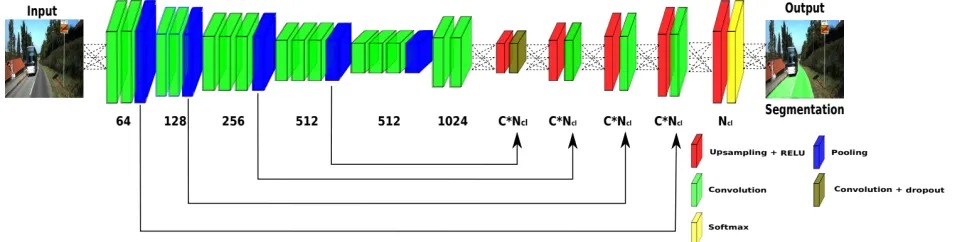
Figure 3: Up-Convolutional Network. The network part up to the first up-sampling layer the encoder side of the network and the following portion the decoder network side. Deconvolution layers have size equal to C∗

Ncl, whereNcl stands for number of classes and C for the scalar factor of filters augmentation. The numbers

under the convolution layers represent the depth. [5]

more memory. Therefore, the most optimal way of training a CNN for road segmentation task is usually via stochas-tic gradient descent (SGD). SGD is a method used during the training phase to reduce the amount of training required while keeping the network better trained by randomly pick-ing samples from a trainpick-ing dataset to train the network.

2.4.2

Dropout

Neural network in general sometimes suffer from overfit-ting. It is condition in which the network is so well trained in the training dataset that it fails to generalize the underlying relationship, causing the network to do poorly in its predic-tion in the testing dataset. This could attributed to the fact that a few weights are trained and modified in the training phase, leaving the rest of the weights effectively deactivated. Therefore, neural networks commonly implements a dropout as a technique to deactivate a certain percentage of weights during the training phase. Doing so would allow the rest of the weights to be trained on the training set, thus allowing the network to better understand the underlying relation-ship of the dataset.

2.5

Fully Convolutional Network

The ultimate goal in road segmentation is that the output of the network has the same size and resolution as the input image with each pixel labeled as road or non-road. As we discussed in section 2.3.3, the pooling layer inside a CNN re-duces the spatial dimension of the input in order to decrease the amount of parameters needed to be trained. Therefore, the end of all pooling and convolution layers results in a se-ries of feature maps that are compressed. In order for the output to match the size and resolution, we need to return these feature maps back to the original input. Long, et al developed a type of CNN called fully convolutional network (FCN) that enables this functionality. An additional layer called deconvolution or up-sample layer is added to the end of a CNN architecture. The deconvolution layer takes in all the feature maps from previous layers and reconstruct the maps back to the size of the input. Another common option that is employed to reconstruct the feature maps back to the original input is through a process called max-unpooling. Max-unpooling preserves the location where the original max-pooling took the maximum value in the spatial

extent considered for max-pooling and pad zeros to all the other empty location, essentially performing a reverse max-pooling operation. The FCN architecture could be general-ized into two main components: encoder anddecoder. The encoder consists of convolutional layers and pooling layers that extract features from images and reduce the spatial di-mension. Meanwhile, the decoder recover the object details and spatial dimensions lost in the encoding component. [4]

3.

METHODS

Oliveira, et al [5] and Caltagirone, et al [2] approach the road segmentation task in two different ways. Oliveira, et al approached the road segmentation problem by creating their own modification of the FCN called Up-Convolution Net-work (Up-Conv-Poly). The Up-Conv-Poly takes in a color road scene image and outputs the same image with the road and non-road surfaces highlighted. Meanwhile, Caltagirone, et al approach the road segmentation problem with their own network called LIDAR-only Deep Neural Network. As the name suggests, it takes in LIDAR point cloud data. The point cloud data is initially 3-dimensional, but then is com-pressed down to a 2-dimensional grid image. The output is similar to the Oliveira, et al network output as it creates the same input image with each grid cell labeled as road or non-road surface.

3.1

KITTI Benchmark Dataset

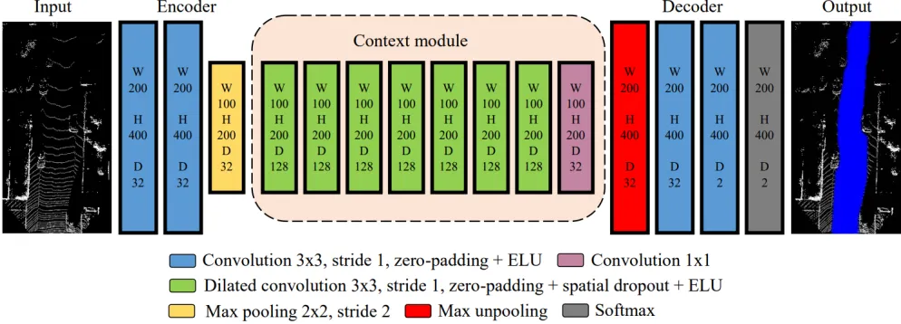
Figure 4: Architecture of the proposed LoDNN. The network has an encoder and a decoder but has an additional implementation of a context module. The input of the network is LIDAR point clouds compressed into 2-dimensional grid. The output has the same dimension and resolution as the input but with road surfaces labeled blue. W represents the width, H represents the height, and D is the number of feature maps. [2]

3.2

Up-Convolutional Network

Up-Convolutional Network takes a color road scene im-age and outputs a class score for each of pixel of the input image, thus labeling each pixel as road or non-road surface. The network like FCNs could be split into two parts, an encoder and a decoder. The encoder is responsible for dis-secting the image for specific features and output a series of feature maps. The encoder part of the network is inherited from a network architecture called Visual Geometric Group (VGG), more information can be found in [7]. Meanwhile, the decoder part of the network adopted the up-sampling layers proposed by Long, et al. The decoder takes in the feature maps generated from the encoder and recreate an output that has the same resolution and spatial dimension as the input. The decoder consists of deconvolution layers that up-samples the features maps via bilinear interpolation. Bilinear interpolation could be summarized as a procedure for taking four data-points in a feature map and using them to construct a larger collection of data-points that brings the spatial dimension closer to the input image.

Dropout layer (discussed in section 2.4.2) is included in the Up-Conv-Poly to avoid overfitting. A convolution layer is implemented right after the up-sampling and convolution layer with the same spatial dimension as the previous layer. This layer is called a 1x1 convolution layer that is designed to increase the amount of non-linearity that can be incorpo-rated into the network [1]. Oliveira, et al also implemented a softmax layer (discussed in section 2.3.4) at the end of network. See figure 3 for a complete architecture design of the Up-Conv-Poly.

Researchers also implemented data augmentation to com-pensate for the small number of training examples. They employ a series of data transformations such as scaling and altering the RGB value of the original image, so that more training examples are available for the network to learn. Thus, increasing the accuracy of the prediction output by the network.

3.3

LIDAR-only Deep Neural Network

Caltagirone, et al developed a LIDAR-only Deep Neural Network (LoDNN) that takes LIDAR point clouds as in-puts and outin-puts a similar result as Up-Conv-Poly. LIDAR point clouds are 3-dimensional point clouds information that needs to be transformed into a suitable format before it can be used as an input for the network. The first step of the procedure is to create a grid in thex-yplane of the LIDAR point clouds and compress the 3-dimensional information into the grid. For each grid cell, some basic statistics are the computed: number of points, mean reflectivity, mean, stan-dard deviation, minimum and maximum elevation. These six grids, each representing an aspect of the original LIDAR point clouds, are then fed into the network.

Like Up-Conv-Poly, LoDNN follows an encoder/decoder configuration. Its encoder is made up of two convolution layers and one pooling layer. The output of the encoder are feature maps that are then passed on to the context module. Context module are made up of dilated convolution layers

which are similar to regular convolution layers but have the receptive field for the filter increasingly expand at every sub-sequent dilated convolution layer. Expanding the size of the filter effectively expands the context for the filter which im-proves accuracy while still keeping the number of parameters down [2]. The activation function used by dilated convolu-tion layers is called an exponential linear unit (ELU). A 1x1 convolution layer is implemented at the end of all dilated convolution layers to add some form of non-linearity into the network. The context module of the network is immedi-ately followed up by the decoder component. The decoder contains a max unpooling layer, followed by two convolu-tion layers and a softmax layer. The two convoluconvolu-tion layers act as up-sampling layers bringing the feature maps gener-ated from the encoder and context module back to the same spatial dimension as the input. See figure 4 for a complete architecture design of the LoDNN.

It was not appropriate to inherit a pretrained encoder

5

Lau: Road Segmentation with Neural Networks

from a previous established network because the encoder would only be trained for camera images. Therefore, Calta-girone, et al deemed it more appropriate to train the network from scratch, using only KITTI training data.

Researchers also implemented data augmentation in their network. Each training images was rotated about the LI-DARz-axis for angles in the range [-30◦, 30◦] using steps of three degrees. After rotation, each example was also mir-rored about x-axis. In this way, the training set was in-creased by a factor of 42. [2]

The output of the network has the same spatial dimension as input grid but with each grid cell labeled as road or non-road surface.

4.

RESULTS

The two proposed networks were both evaluated on the KITTI road benchmark test set in the urban road category. Some metrics were used for evaluation such as recall (REC), precision (PRE), maximum F1-measure (MaxF), and time it took to make inference on a single image. Four important metrics are also needed to considered, true positives (TP), representing the road surfaces predicted by the network was accurate; false positives (FP), representing the road sur-faces predicted by the network was inaccurate; true nega-tives (TN), representing the non-road surfaces predicted by the network was accurate; false negatives (FN), representing the non-road surfaces predicted by the network was inaccu-rate. Given the definitions of the four important metrics, we can now understand what precision and recall means,

P recision= T P

T P+F P Recall = T P T P+F N

Precision is also a statistical term that determines how much of the road surfaces determined by the network was actually accurate out of all road surfaces determined by the network. Recall is a statistical term that determines how much of the road surfaces determined by the network was actually accurate out of all possible road surfaces in the in-put image. The maximum F1-measure is the harmonic aver-age between the recall and precision. Table 1 illustrates the performance result gathered from both Up-Conv-Poly and LoDNN after running the road benchmark test set.

Table 1: KITTI Road Benchmark Results (In %) On Urban Road Category

Method MaxF REC PRE Time (ms) LoDNN [2] 94.07 95.37 92.81 18 Up-Conv-Poly [5] 93.83 93.67 94.00 80

LoDNN outperformed Up-Conv-Poly in terms of the max-imum F1-measure, precision and inference time, meaning LoDNN has a higher accuracy and was faster than Up-Conv-Poly in making predictions on new images. Caltagirone, et al did not explain the exact reason why LoDNN received a higher accuracy and less inference time. But judging from the differences in the network architecture and types of in-put, one might be able to deduce that LIDAR systems could ignore much of the background noises (shadows, light reflec-tion, etc) compared to camera images. One thing to notice

that Up-Conv-Poly did receive a higher precision in its net-work than LoDNN did. Although, no explanations were given as to why this has occurred. Thus, it propagated the effect to the network in which less work is needed by the network to make inference and increasing the accuracy of its inference.

5.

CONCLUSION

As demonstrated by the work of Oliveira, et al. and Cal-tagirone, et al. neural networks show considerable promises in road segmentation in terms of their accuracy in predict-ing road surface and performance. Oliveira, et al. combined previous trained encoder from [7] and the up-sampling lay-ers from [4] to create the Up-Conv-Poly. Meanwhile, Cal-tagirone, et al trained its own encoder and implemented a context module to increasingly expand the receptive field of its convolution layers, thus increasing the context con-sidered by the filters. When comparing the performance of each network, the LoDNN came out ahead in terms of its harmonic average of precision and accuracy as well as its inference time of the KITTI road data set in the urban road category.

Acknowledgments

Many thanks to my advisor, Peter Dolan, my professor for senior seminar, Elena Machkasova, and my alumnus reviewer, Mitchell Finzel, for your guidance and feedback.

6.

REFERENCES

[1] Cs231n convolutional neural networks for visual recognition.http://cs231n.github.io/. Accessed: 2018-03-20.

[2] L. Caltagirone, S. Scheidegger, L. Svensson, and M. Wahde. Fast lidar-based road detection using fully convolutional neural networks. In2017 IEEE Intelligent Vehicles Symposium (IV), pages 1019–1024, June 2017. [3] C. John and C. Scott. A survey of lidar technology and

its use in spacecraft relative navigation. 2013. [4] J. Long, E. Shelhamer, and T. Darrell. Fully

convolutional networks for semantic segmentation. In

2015 IEEE Conference on Computer Vision and Pattern Recognition (CVPR), pages 3431–3440, June 2015.

[5] G. L. Oliveira, A. Valada, C. Bollen, W. Burgard, and T. Brox. Deep learning for human part discovery in images. In2016 IEEE International Conference on Robotics and Automation (ICRA), pages 1634–1641, May 2016.

[6] B. Ranft and C. Stiller. The role of machine vision for intelligent vehicles.IEEE Transactions on Intelligent Vehicles, 1(1):8–19, March 2016.

[7] K. Simonyan and A. Zisserman. Very deep convolutional networks for large-scale image recognition.CoRR, abs/1409.1556, 2014.