Unsteady Three-Dimensional MHD Dusty Couette Flow through Porous Plates with Heat Source

(1)

Vol. 4, No. 2, 2016, 59-76 ISSN: 2321 – 9238 (online) Published on 28 September 2016

www.researchmathsci.org

59

Progress in

Unsteady Three-Dimensional MHD Dusty Couette Flow

through Porous Plates with Heat Source

C.Loganathan1 and S.Gomathi2 1

Department of Mathematics, Maharaja Arts and Science College Coimbatore- 641014, India. E-mail: [email protected] 2

Department of Mathematics, Maharaja Arts and Science College Coimbatore- 641014, India. E-mail:[email protected]

Received 12 September 2016; accepted 27 September 2016

Abstract. The unsteady three-dimensional Couette flow of a viscous incompressible fluid

between two porous flat plates with uniform injection and periodic suction in the presence of magnetic field, radiation and heat source/sink has been investigated. Perturbation technique has been used to obtain approximate solutions for the velocity and temperature fields, skin friction and Nusselt number. The velocity and temperature profiles have been plotted to study the effects of heat parameter, Hartmann number and other non-dimensional parameters on them. Furthermore, skin friction and Nusselt number have been tabulated for different values of the non-dimensional parameters.

Keywords: Slip flow regime, MHD, heat source, porous medium, Couette flow, dusty

fluid

1. Introduction

Dusty Couette flows in the presence of magnetic field finds its application in many industrial processes in the field of aerodynamics, nuclear cooling and geophysics. Some of their applications include liquid metal cooling of nuclear reactors, electromagnetic casting and plasma confinement. The steady two-dimensional plane Couette flow with transpiration cooling for uniform injection and suction at the porous plates for a clear fluid has been discussed in Eckert [7].

Raptis [2] studied the steady two dimensional free convection flow through a very porous medium subjected to a constant suction velocity and bounded by a vertical infinite porous plate in the presence of radiation. The flow velocity was found to be increasing with the radiation parameter. Seddeek [15] investigated the effect of variable viscosity on free convective flows with magnetic field and radiation. The solutions were obtained using the shooting method and similarity solutions.

(2)

60

temperature was analysed by Pathak and Maheshwari [9]. The analytical solution of resulting ordinary differential equations was obtained in terms of repeated integrals of complementary error functions.

The steady three dimensional Couette flow with uniform suction at the stationary plate and transverse sinusoidal injection at the uniformly moving plate has been studied by Sharma et al. [5] to study the effects of Prandtl number, radiation parameter and injection parameter on the rate of heat transfer. The unsteady Couette flow of an electrically conducting, viscous, incompressible fluid bounded by two parallel non-conducting porous plates with uniform suction and injection in the presence of transverse magnetic field was studied with heat transfer by Attia [10]. The effects of magnetic field and uniform injection and suction was examined on the velocity and temperature fields.

Loganathan and Prathiba [6] studied the effect of uniform magnetic field on a viscous, incompressible fluid past a spherical and permeable aggregate. Jump boundary conditions were used at the interface between the porous region and clear fluid. The magnetic field with variable permeability is found to effect the stress jump coefficient which changes the normalized drag and torque. Baoku et al. [11] investigated the effects of thermal radiation and magnetic field on hydromagnetic Couette flow of a highly viscous fluid with temperature-dependent viscosity and thermal conductivity at constant pressure through a porous channel. The relevant governing partial differential equations were transformed to non-linear coupled ode and solved numerically using a marching finite difference scheme to obtain the velocity and temperature profiles. The magnetohydrodynamic flow of viscous incompressible fluid past a vertical porous plate in the presence of radiation was analysed by Guria et al. [13]. The main fluid velocity was found to decrease with increase in Hartmann number, radiation parameter as well as suction parameter for cooling of the plate and increase for heating of the plate.

Radiation effects on free convection MHD Couette flow started exponentially with variable wall temperature in the presence of heat generation were investigated by Das et al. [16]. The governing equations were solved analytically using the Laplace transform technique and the variations of velocity and fluid temperature were analysed. Unsteady MHD couette flow between two infinite parallel porous plates in an inclined magneticfield with heat transfer were studied by Joseph et al. [12]. The governing equations were solved by variable separable technique to study the effects of various parameters such as Hartman number and Prandtl number on the flow field.

Jha et al. [3] investigated the unsteady MHD free convective Couette flow of viscous incompressible electrically conducting fluid between two infinite vertical porous plates in the presence of transverse magnetic field and thermal radiation. Solutions for time dependent energy and momentum equations were obtained by the implicit finite difference method and verified by steady state solutions obtained by using the perturbation method. Similar method was applied by Jha et al. [4] to study the combined effect of injection/suction.

(3)

61 2. Flow description and governing equations

The flow under investigation has been modelled as an unsteady three dimensional flow of a viscous, incompressible, dusty fluid between two horizontal porous flat plates separated by a distance ‘d’ in a slip flow regime with uniform suction at the stationary plate and periodic suction at the plate in motion. A uniform magnetic field is applied to the plate as shown in Fig. 1.

Figure 1: Couette dusty flow with constant injection and periodic suction at the porous plates.

The upper plate is assumed to be the one in motion with uniform velocity in the direction of the flow. The Cartesian coordinate system is chosen with its origin on the lower stationary plate, ∗- axis in the direction of the flow, ∗- axis taken perpendicular to the plate and directed into fluid flowing in laminar regime with a uniform free stream velocity and ∗- axis is taken normal to the ∗∗- plane.

The upper plate is subjected to a constant injection − and the lower plate to a transverse sinusoidal time dependent suction velocity distribution of the form

∗₌_−V_{1 + ε cos}∗

∗ − ct∗ (1)

where ≪ 1 is the amplitude of the suction velocity as shown in Fig 2.1. The distance between the plates is taken equal to the suction velocity. The slip condition is assumed for the fluid phase and similar slip condition is also assumed for the particle phase.

Denoting dimensional velocity components as ∗, ∗ and ∗ in the directions ∗,

∗_and∗_{axes respectively for the fluid phase,} ! ∗_,

!∗ and _!∗ in the directions ∗, ∗ and

x∗

y∗

z∗

T T&

u∗

B

y∗_{= d}

y∗_{= 0}

SV

(4)

62

∗_{axes respectively for the particle phase and}_-∗_and

-!∗ for the temperature of the fluid and particle phase respectively, the governing equations are given as:

For fluid phase:

./∗

.0∗+ .1 ∗

.2∗ = 0 (2)

.3∗

.4∗+ ∗ .3 ∗

.0∗+ ∗ .3 ∗

.2∗ = 5 . 6₃

.0∗6+ . 6₃

.2∗6 + 789-∗− -:∗ −;<= 6₃∗

> +

?@=

> A!∗− ∗B (3)

./∗

.4∗+ ∗ ./ ∗

.0∗+ ∗ ./ ∗

.2∗ = 5 . 6_/

.0∗6+ . 6_/

.2∗6 +.! ∗

.0∗+ ?@_>=A!∗− ∗B (4)

.1∗

.4∗ + ∗ .1 ∗

.0∗+ ∗ .1 ∗

.2∗ = 5 . 6₁

.0∗6+ . 6₁

.2∗6 +.! ∗

.2∗−;<= 6₁∗

> +

?@=

> A !∗− ∗B (5)

CD!.9

∗

.4∗+ ∗ .9 ∗

.0∗+ ∗ .9 ∗

.2∗ = E . 6₉

.0∗6+ . 6₉

.2∗6 −.F_.0G∗+ H-∗− - + >IJK

LM A!

∗₋∗_B ₍₆₎

For particle phase:

./I∗

.0∗+ .1_.2I∗∗ = 0 (7)

.3I∗

.4∗+ !∗ .3_.0I∗∗+ !∗ .3_.2I∗∗ = _N?_IA∗− !∗B (8)

./I∗

.4∗+ !∗ ./_.0I∗∗+ !∗ ./_.2I∗∗ = _N?_IA∗− !∗B (9)

.1I∗

.4∗ + !∗ .1_.0I∗∗+ !∗ .1_.2∗I∗ = _N?_IA ∗− !∗B (10)

.9I∗

.4∗+ !∗ .9_.0I∗∗+ !∗ .9_.2I∗∗ = _LO_IA-∗− -!∗B (11)

The corresponding boundary conditions are:

∗_{= P} O ∗ .3∗

.0∗ ; ∗= −V1 + ε cos ∗

∗ − ct∗; ∗= P∗ .1O ∗

.0∗ ; -∗= -+ PQ∗ .9 ∗

.0∗ ; !∗ = P∗ .3O_.0I∗∗; !∗= −V1 + ε cos

∗

∗ − ct∗; !∗= PO∗ .1_.0I∗∗ ; -!∗= -+ P∗ .9Q ∗

.0∗

at = 0 (12)

∗₌_;_!∗_{= −V}_; ∗_{= 0}_;_-∗_{= -}_O_;_!∗ ₌_;_!∗_{= −V}_; _!∗_{= 0}_;_-_!∗_{= -}_O

at = R (13)

where P∗_O= QST_T P, P_Q∗ = QST_T PU and P = V _QX>W O QY is the mean free path and Z is the Maxwell's reflection coefficient.

(5)

63

.FG∗

.0 = 4-∗− -\ (14)

where

\ = ] ^_{_}₌.`_.9ab

Rc d

(15)

By introducing the following non-dimensional parameters:

= 0_:∗ ; = 2_:∗ ; e = fe∗; g = _>h!∗

=6 ; =

3∗

i ; = /∗

h= ; =

1∗

h= ; j =

9∗_S9 k∗

9₌∗_S9 k∗ ; Γ!=m:_h₌; _! =3_iI∗ ; _! =/_hI∗

= ; !=

1I∗

h= ; j! =

9I∗S9k∗

9₌∗_S9

k∗ ; Reynolds number no =

h=:

p ;

Prandtl number qZ =rJ_sI ; Mass concentration parameter t =@=_>N ; Slip parameter

ℎ =_:v ; Grashof number wZ =xyM:A9_ih=∗S9k∗B

= ; Frequency parameter c =

z:6

p ; Relaxation

time parameter Λ =N_:?Ih= ; Hartmann number | =;<_r=6:6 ; Radiation parameter }_O=

~:6

rJI; Heat source parameter }Q=

:6

rJI; Heat parameter } = }O− }Q.

(16) The governing equations (2-13) can be rewritten in non-dimensional form as follows:

./ .0+

.1

.2 = 0 (17)

c.3_.4+ no .3_.0+ .3_.2 = _.0.63₆+._.263₆ + nowZj − | +`_m A_!− B (18)

c./_.4+ no ./_.0+ _.2./ = _.0.6/₆+._.26/₆ − no.!_.0+`_m A_!− B (19)

c.1_.4 + no .1_.0+ .1_.2 = ._.061₆+._.261₆ − no.!_.2− | +`_m A _!− B (20)

cqZ._.4 + noqZ ._.0+ ._.2 = ._.06₆+._.26₆ − }noqZj +Q`_m Aj_!− jB (21)

./I

.0 + .1I

.2 = 0 (22)

c.3I

.4 + no ! .3I

.0 + ! .3I

.2 = `mA − !B (23)

c./I

.4 + no ! ./I

.0 + ! ./I

.2 =

`

m A − !B (24)

c.1I

.4 + no ! .1I

.0 + ! .1I

.2 = `m A − !B (25)

c.I

.4 + no ! .I

.0 + ! .I

.2 =

`

m Aj − j!B (26)

The corresponding boundary conditions are:

= ℎO.3_.0 ; = −S1 + ε cosπz − t; = ℎ_O.1_.0 ; j = ℎ_Q._.0;

!= ℎO.3_.0I ; _!= −S1 + ε cosπz − t; _! = ℎ_O.1_.0I ; j_!= ℎ_Q._.0I

(6)

64

= 1; = −S; = 0 ; j = 1 ; _! = 1 ; _!= −S; _! = 0 ; j_! = 1

at = 1 (28)

3. Solution of the problem When the amplitude of oscillation in the suction velocity is small ≪ 1, we can assume , , , j, _!, _!, _!, j_! and g in the following form to solve the differential equations (17)-(26). , , e = + _O, , e + Q_Q, , e + ⋯ , , e = + _O, , e + Q_Q, , e + ⋯ , , e = + _O, , e + Q _Q, , e + ⋯ j, , e = j + j_O, , e + Qj_Q, , e + ⋯ !, , e = _! + _!O, , e + Q_!Q, , e + ⋯ !, , e = _! + _!O, , e + Q_!Q, , e + ⋯ !, , e = _! + _!O, , e + Q _!Q, , e + ⋯ j!, , e = j_! + j_!O, , e + Qj_!Q, , e + ⋯ g, , e = g + g_O, , e + Qg_Q, , e + ⋯ (29)

When = 0, the differential equations pertaining to two dimensional flow are obtained as: U = 0 (30)

UU− noU + nowZj− |+`_m _!− = 0 (31)

gU = _m_!− (32)

UU− no U − | +`_m _!− = 0 (33)

jUU− noqZjU− qZ}j+Q`_m j_!− j = 0 (34)

_!U ₌ _{0 (35)}

_!U +O_m_!− = 0 (36)

_! = (37)

_!U +_mO _!− = 0 (38)

j_!U +O_mj_!− j = 0 (39)

Subject to the boundary conditions: = ℎO.3_.0= ; = −; = ℎ_O.1_.0= ; j= ℎ_Q._.0= ; _!= ℎO.3_.0I= ; _!= −S; _!= ℎ_O.1_.0I= ; j_!= ℎ_Q._.0I= at = 0 (40)

(7)

65

The solutions for the equations (30), (32), (35) and (37) are

= _! = − (42)

gU ₌ ₀ ₍₄₃₎

Substituting equations (42) and (43) in the remaining equations and rearranging as done in Govindarajan et al. [1], we get

−ΛSUUU+ 1 − noΛQUU+ no1 + t + Λ|U − | =

−nowZj+ ΛnowZjU (44)

−ΛS UUU+ 1 − noΛQ UU+ no1 + t + Λ| U− | =0 (45)

−ΛSjUUU+ 1 − noqZΛQjUU+ no qZ +Qt + ΛqZ} jU − qZ}j =0 (46)

−ΛS_!U ₊

! = (47)

−ΛS _!U ₊

! = (48)

−ΛSj_!U + j_! = j (49)

The solution to the remaining equations are:

= _! = 0 (50)

j = _Oo0+ _Qo60+ o0₍₅₁₎ j_! = _~o0+

OSmo

0+ 6

OSm6o

60+

OSmo

0₍₅₂₎ = o0+ _Oo0+ _OOo0+ _OQo0+ _Oo60+ _O~o0₍₅₃₎ _! = _Oo0+ _Oo0+ _Oo0+ _Oo0+ _Oo0+ _Qo60+

QOo0 (54) The unsteady state equations of first order are:

./

.0 + .1

.2 = 0 (55)

c.3

.4 + no − .3

.0 + O .3=

.0 = .6₃

.06 +. 6₃

.26 + nowZjO− |O+ `_m _!O− O (56)

c./

.4 + no − ./

.0 =

.6_/

.06 +. 6_/

.26 − no.!_.0+

`_m _!O− O (57)

c.1

.4 + no −.1.0 = .

6₁

.06 +. 6₁

.26 − no.!_.2− | O+ `_m _!O− O (58)

cqZ.

.4 + noqZ −..0+ O..0= = .

6

.06 +. 6

.26 − qZ}j +

Q`_m j_!O− jO (59)

./_I .0 +

.1_I

(8)

66

c.3I

.4 + no − .3_I

.0 + !O .3_I=

.0 = `m O− !O (61)

c./_.4I+ no −./_.0I = `_m _O− _!O (62)

c.1_.4I+ no −.1_.0I = `_m _O− _!O (63)

c.I

.4 + no − ._I

.0 + !O ._I=

.0 =

`

mjO− j!O (64)

The boundary conditions become

O= ℎO.3_.0 ; _O= −SAf − eB; _O= ℎ_O.1_.0 ; j_O= ℎ_Q._.0 ;

_!O= ℎO.3_.0I ; _!O= −SAf − eB ; _!O= ℎ_O.1_.0I ; j_!O= ℎ_Q._.0I at = 0 (65)

O= O= O= jO= _!O= _!O= _!O= j_!O= 0 at = 1 (66)

In order to solve these partial differential equations _O, _O, _O, j_O, _!O, _!O, _!O, j_!O and g_O are assumed to be of the following complex form:

O, , e = _OOoW2S4

O, , e = OOoW2S4

O, , e = _W_OOU oW2S4

jO, , e = j_OOoW2S4

_!O, , e = _!OOoW2S4

!O, , e = _W_!OOU oW2S4

j_!O, , e = j_!OOoW2S4

gO, , e = g_OOoW2S4

(67) Now using (67) in equations (55)-(64) and rearranging as before, we get

OOUU + noOOU + −Q+ c − |OO+`_m _!OO− OO =

−nowZjOO+ noOOU (68)

OOUU + noOOU + −Q+ cOO+`_m _!OO− OO = nogOOU (69)

_OOUUU_{+ no}

OOUU + −Q+ c − |OOU +`_m _!OOU − OOU = QnogOOU

(70)

jOOUU + noqZjOOU + −Q+ cqZ − qZ}jOO+Q`_m j_!OO− jOO

= no_OOjU (71)

−Λ_!OOU _{+ 1 −}_m

(9)

67

−Λ_!OOU _{+ 1 −}_m

` !OO = OO (73)

−Λ_!OOUU _{+ 1 −}_m

` !OOU = OOU (74)

−Λj_!OOU + 1 −_m_` j_!OO = j_OO− Λ_!OOj_!U (75)

Boundary conditions are

OO= ℎO.3_.0 ; OO= −; _OO= ℎ_O.1_.0 ; j_OO= ℎ_Q._.0 ;

_!OO = ℎO.3_.0I; _!OO= −; _!OO= ℎ_O.1_.0I ; j_!OO= ℎ_Q._.0I

at = 0 (76)

OO= OO= OO= jOO= _!OO = _!OO= _!OO= j_!OO= 0 at = 1 (77)

The solutions of the equations (68)-(75) subject to boundary conditions (76)-(77) are

OO = _Oo¡0+ _Qo¢0+ o=0+ _~o0+ o60+ o0₍₇₈₎ _!OO = o0+ o¡0+ o¢0+ _Oo=0+ _OOo0+ _OQo60+

Oo0 (79)

OO = _W_O£o¡0+ _Q£o¢0+ £_Oo=0+ _~£_OOo0+ o60+

£Oo0 (80)

!OO = _W¤£O~o

0+ £o¡0+ £o¢0+ _O£_Oo=0

+OO£OOo0+ OQ£OQo60+ O£Oo0 ¥ (81)

jOO = D_Oo0+ D_Qo0+ Do0+ (D_~o¡0+ Do¢0+ Do=0+

Do0+ Do60 + Do0+ DOo0) o0+ (D_OOo¡0+

DOQo¢0+ DOo=0+ DO~o0+DOo60+ DOo0+

DOo0o60 +(D_Oo¡0+ D_Oo¢0+ D_Qo=0+ D_QOo0₊ DQQo60+ DQo0+ DQ~o0o0+ DQo¡0+ DQo¢0+

DQo=0+ DQo0+ DQo60+ Do0+ DOo0 o0 (82)

j_!OO = D_Qo0+ Do0+ D_~o0+ Do0+ Do¡0+

Do¢0+ Do=0+ Do0+ D~o60 + D~Oo0+

D~Qo0) o0+₍D_~o¡0+ D_~~o¢0+ D_~o=0+ D_~o0+ D~o60+ D~o0+ D~o0 ) o60+ Do¡0+ DOo¢0+

DQo=0+ Do0+ D~o60+ Do0+ Do0 o0+

(Do¡0+ Do¢0+ Do=0+ Do0+ D_Oo60+

DQo0+ Do0 o0 (83)

OO = ¦_Oo¡0+ ¦_Qo¢0+ ¦o6=0+ ¦_~o0+ ¦o0+ ¦o0+ (¦o¡0+ ¦o¢0+ ¦o=0+ ¦_Oo0+ ¦_OOo60+ ¦_OQo0+

(10)

68

¦_Qo=0+ ¦_Q~o0+ ¦_Qo60+ ¦_Qo0+ ¦_Qo0) o0+ (¦_Qo¡0+ ¦_Qo¢0+ ¦o=0+ ¦_Oo0+ ¦_Qo60+

¦o0+ ¦~o0 o0+(¦o¡0+ ¦o¢0+ ¦o=0+ ¦o0+ ¦o60+ ¦~o0+ ¦~Oo0 o0+(¦_~Qo¡0+ ¦~o¢0+ ¦~~o=0+ ¦~o0+ ¦~o60+ ¦~o0+

¦~o0o0+ ¦~o¡0+ ¦o¢0+ ¦Oo=0+ ¦Qo0+

¦o60+ ¦~o0+ ¦o0 o0 (84)

_!OO = ¦o0+ ¦o¡0+ ¦o¢0+ ¦o6=0+ ¦o0+

¦Oo0+ ¦Qo0+ ¦o¡0+ ¦~o¢0+ ¦o=0+

¦o0+ ¦o60+ ¦o0+ ¦o0 o0+ ¦o¡0+

¦Oo¢0+ ¦Qo=0+ ¦o0+ ¦~o60+ ¦o0+

¦o0 o60+ ¦o¡0+ ¦o¢0+ ¦o=0+ ¦o0+

¦Oo60+ ¦Qo0+ ¦o0 o0+ ¦~o¡0+ ¦o¢0+

¦o=0+ ¦o0+ ¦o60+ ¦o0+ ¦o0 o0+

(¦_Oo¡0+ ¦_Qo¢0+ ¦o=0+ ¦_~o0+ ¦o60+ ¦o0+ ¦o0 o0+ ¦o¡0+ ¦o¢0+ ¦Oo=0+

¦OOo0+ ¦OQo60+ ¦Oo0+ ¦O~o0 o0+

¦Oo¡0+ ¦Oo¢0+ ¦Oo=0+ ¦Oo0+ ¦Oo60+

¦OOo0+ ¦OOOo0 o0 (85)

Skin friction

The skin friction at the wall due to main flow is given by:

§¨ = :3_:0

0© =

:3=

:0_0©+ :3

:0 _0©oW2S4+ ΟQ

= §₃₌+ no_¨cos − e + «_¨ (86)

The skin friction at the wall due to cross flow is given by:

§2 = :1_:0

0© =

:1=

:0_0©+ :1

:0 _0©oW2S4+ ΟQ

= no₂cos − e + «₂ (87)

Nusselt number

The rate of heat transfer from the plate can be calculated using the formula

¬1= − .9_.0

0© and can be written in non-dimensional form as Nusselt number:

= − :_:0

0© = − :=

:0_0©− :

:0_0©oW2S4+ ΟQ

= −jU0 + no₉cos − e + «₉ (88)

4. Numerical results

(11)

69

and Nusselt number have been tabulated (Table 1-4) for different values of non-dimensional parameters such as Grashof number (Gr), Reynolds number (Re), Prandtl number (Pr), heat parameter (F), mass concentration parameter (f), relaxation time parameter (Λ_{), suction parameter (S), temperature slip parameter (h2) and Hartmann}

number (M).

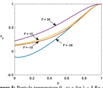
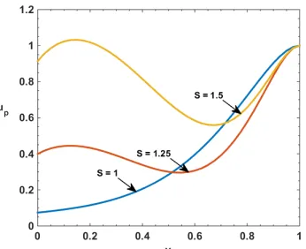
Increasing the Hartmann number (M) results in an increase in the main velocity magnitude for both fluid and particle phase (Fig 2-3) but it has little effect on the cross flow velocity. An increase in the suction parameter (S) results in circulation in the flow profiles and the main flow velocity also increases for both the phases (Fig 12-13). A similar trend is also observed with the cross-flow velocity profile as expected for increasing suction parameter (Fig 8-9). The fluid and particle temperature profiles increase with increasing value of the temperature slip parameter (Fig 6-7). For the increasing heat parameter, the temperature profiles were also found to be increasing for both fluid and particle phases (Fig 4-5).

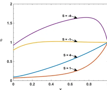
The temperature profiles for the fluid phase when suction parameter are +1 and -1 are as expected. For both the cases, increasing the magnitude of suction parameter results in an increase in the over all temperature of the fluid (Fig 10). The particle temperature profiles were found to be more uniformly increasing with increasing suction parameter magnitude. This is because increasing the suction parameter results in a decrease in relaxation time for the phases thereby resulting in a more uniform cooling/heating depending on the sign of the suction parameter (Fig 11).

The amplitude of the shear stress and the tangent of phase shift due to main flow decreases with the increasing Hartmann number (M) (Table 1). For the increasing suction parameter (S), there is no clear trend in the amplitude of shear stress or the magnitude of tangent of phase shift due to main flow (Table 1). On the other hand, the amplitude of the shear stress and the tangent of phase shift due to the cross flow velocity increases with increasing suction parameter (S) as seen in Table 2.

The amplitude of Nusselt number and the amplitude of the tangent of the phase shift are found to increase with the increasing magnitude of the heat parameter (F) as seen from Table 3. The amplitude of Nusselt number is found to be decreasing for F>0 and increasing for F<0 but there is no clear trend for the tangent of phase shift (Table 3).

The amplitude of Nusselt number decreases with increasing values of the temperature slip parameter (h2) but there is little effect on the tangent of the phase shift (Table 4).

5. Conclusion

We have extended the work of Guria [14] to study the effect of dust particles and the magnetic and heat parameter with slip condition on the three dimensional unsteady couette flow of viscous incompressible fluid between two horizontal porous flat plates. A periodic suction is applied to the stationary plate and a constant injection is applied to the uniformly moving plate. The conclusions of the study are:

Increasing the Hartmann number (M) increases the main flow velocity for both fluid and particle phase.

Hartmann number (M) has little effect on the cross flow velocities.

(12)

70

The fluid and particle temperature profiles increase with increasing value of the temperature slip parameter (h2).

The particle temperature profiles were found to be more uniformly increasing with increasing suction parameter magnitude.

The amplitude of the shear stress and the tangent of phase shift due to main flow decreases with the increasing Hartmann number (M).

The amplitude of Nusselt number and the amplitude of the tangent of the phase shift are found to increase with the increasing magnitude of the heat parameter (F).

Figure 2: Main velocity u vs y for λ_{= 5, Re = 5, Gr}

= 5, Pr = 0.71, S = 1, F = 1, h1 = 0.5, h2 = 0.5, f = 0.2,Λ_{= 0.2,z = 0.0, t = 0.0,}ε_{= 0.05}

Figure 3: Main particle velocity up vs y for λ = 5, Re = 5, Gr = 5, Pr = 0.71, S = 1, F = 1, h1 = 0.5, h2 = 0.5, f = 0.2, Λ_{= 0.2, z = 0.0, t = 0.0,}ε_{= 0.05}

Figure 4: Temperature θ_{vs y for}λ_{= 5, Re = 5, Gr =}

5, Pr = 0.71, S = 1, M = 1, h1 = 0.5, h2 = 0.5, f = 0.2,

Λ_{= 0.2, z = 0.0, t = 0.0,}ε_{= 0.05}

Figure 5: Particle temperature θ

(13)

71

Figure 6: Temperature θ_{vs y for}λ_{= 5, Re = 5, Gr =}

5, Pr = 0.71, S = 1, M = 1, F = 1, h1 = 0.5, f = 0.2, Λ

= 0.2, z = 0.0, t = 0.0, ε_{= 0.05}

Figure 7: Particle temperature θ_{p vs y for}λ_{= 5, Re}

= 5, Gr = 5, Pr = 0.71, S = 1, M = 1, F = 1, h1 = 0.5, f = 0.2, Λ_{= 0.2, z = 0.0, t = 0.0,}ε_{= 0.05}

Figure 8: Cross-flow velocity w vs y for λ_{= 5, Re =}

5, Gr = 5, Pr = 0.71, M = 1, F = 1, h1 = 0.5, h2 = 0.5, f = 0.2, Λ_{= 0.2, z = 0.0, t = 0.0,}ε_{= 0.05}

Figure 9: Cross-flow particle velocity wp vs y for λ = 5, Re = 5, Gr = 5, Pr = 0.71, M = 1, F = 1, h1 = 0.5, h2 = 0.5, f = 0.2, Λ_{= 0.2, z = 0.0, t = 0.0,}ε_{= 0.05}

Figure 10: Temperature θ_{vs y for}λ_{= 5, Re = 5, Gr}

= 5, Pr = 0.71, M = 1, F = 1, h1 = 0.5, h2 = 0.5, f = 0.2, Λ_{= 0.2, z = 0.0, t = 0.0,}ε_{= 0.05}

Figure 11: Particle temperature θ

(14)

72

Figure 12: Main flow velocity u vs y for λ_{= 5, Re =}

5, Gr = 2.5, Pr = 0.71, M = 1, F = 1, h1 = 0.5, h2 = 0.5, f = 0.2, Λ_{= 0.2, z = 0.0, t = 0.0,}ε_{= 0.05}

Figure 13: Main flow particle velocity u p vs y for λ

= 5, Re = 5, Gr = 2.5, Pr = 0.71, M = 1, F = 1, h1 = 0.5, h2 = 0.5, f = 0.2, Λ_{= 0.2, z = 0.0, t = 0.0,}ε₌

0.05

Table 1: Shear stress due to main flow at y = 0 for λ_{= 5, Re = 2, Gr = 5, Pr = 0.71, F = 1,}

h1 = 0.5, h2 = 0.5, f = 0.2, Λ_{= 0.2, z = 0.0, t = 0.0,}ε_{= 0.05.}

S no_¨ tan «_¨

M = 1 M = 5 M = 10 M = 1 M = 5 M = 10

1 0.0802 0.4325 0.2901 -0.1182 -0.2760 -4.8287

1.25 59.6476 1.6503 1.4687 -2.5139 -0.8443 -0.8526

1.5 26.2496 1.9640 1.4572 -2.5800 0.6884 -0.2186

Table 2: Shear stress due to cross flow at y = 0 for λ_{= 5, Re = 2, Gr = 5, Pr = 0.71, M =}

1, F = 1, h1 = 0.5, h2 = 0.5, f = 0.2, Λ_{= 0.2, z = 0.0, t = 0.0,}ε_{= 0.05.}

S no₂ tan «₂

1 0.9161 -0.8255

1.25 0.9591 -0.6211

1.5 1.0096 -0.3926

Table 3: Nusselt number at y = 0 for λ_{= 5, Re = 2, Gr = 5, Pr = 0.71, M = 1, h1 = 0.5, h2}

= 0.5, f = 0.2, Λ_{= 0.2, z = 0.0, t = 0.0,}ε_{= 0.05.}

F no₉ tan «₉

S = 1 S = 1.25 S = 1.5 S = 1 S = 1.25 S = 1.5

30 60.7026 41.7222 4.1472 -0.4293 -2.9963 -0.6552

0 0.0969 0.6256 1.1400 -0.2994 0.0486 0.4655

-30 0.0953 0.6303 0.9268 -44.4020 0.0705 0.3132

Table 4: Nusselt number at y = 0 for λ_{= 5, Re = 2, Gr = 5, Pr = 0.71, M = 1, F = 1, S =}

1, h1 = 0.5, f = 0.2, Λ_{= 0.2, z = 0.0, t = 0.0,}ε_{= 0.05.}

h2 no₉ tan «₉

0 0.7102 -0.5908

2 0.2292 -0.6000

(15)

73 REFERENCES

1. A.Govindarajan, V.Ramamurthy and K.Sundarammal, 3D Couette flow of dusty fluid with transpiration cooling, Journal of Zhejiang University SCIENCE A, 8 (2007) 313-322.

2. A.Raptis, Radiation and free convection flow through a porous medium,

International Communications in Heat and Mass Transfer, 25 (1998) 289-295. 3. B.K.Jha, B.Y.Isah and I.J.Uwanta, Unsteady MHD free convective Couette flow

between vertical porous plates with thermal radiation, Journal of King Saud

University, 27 (2015) 338-348.

4. B.K.Jha, B.Y.Isah and I.J.Uwanta, Combined effect of suction/injection on MHD free-convection flow in a vertical channel with thermal radiation, Engineering

Physics and Mathematics, (2016).

5. B.K.Sharma, M.Agarwal and R.C.Chaudhary, Radiation effect on temperature distribution in three-dimensional Couette flow with suction or injection, Applied

Mathematics and Mechanics, 28 (2007) 309-316.

6. C.Loganathan and S.R.Prathiba, Magnetohydrodynamic flow past a porous spherical aggregate with stress jump conditions, Progress in Nonlinear Dynamics and Chaos, 1 (2013) 76-92.

7. E.R.G.Eckert, Heat and Mass Transfer, McGraw-Hill, New York, 1958.

8. G.Bodosa and A.K.Borkakati, MHD Couette flow with heat transfer between two horizontal plates in the presence of a uniform transverse magnetic field, Theoretical

Applied Mechanics, 30 (2003) 1-9.

9. G.Pathak and C.H.Maheshwari, Effect of radiation on unsteady free convection flow bounded by an oscillating plate with variable wall temperature, International Journal

of Applied Mechanics and Engineering , 11 (2006) 371-382.

10. H.A.Attia, Unsteady MHD couette flow with heat transfer in the presence of uniform suction and injection, Mechanics and Mechanical Engineering, 12 (2008) 165-176.

11. I.G.Baoku, G.Israel-Cookey and B.I.Olajuwon, Magnetic field and thermal radiation effects on steady hydromagnetic Couette flow through a porous channel, Surveys in

Mathematics and its Applications, 5 (2010) 215-228.

12. K.M.Joseph, S.Daniel and G.M.Joseph, Unsteady MHD couette flow between two infinite parallel porous plates in an inclined magnetic field with heat transfer,

International Journal of Mathematics and Statistics Invention, 2 (2014) 103-110. 13. M.Guria, N.Ghara and R.N.Jana, Radiation effect on three dimensional mhd flow

past a vertical porous plate, Journal of Physical Sciences, 15 (2011) 161-170.

14. M.Guria, Effect of slip condition on vertical channel flow in the presence of radiation, International Journal of Applied Mechanics and Engineering, 21 (2016) 341-358.

15. M.A.Seddeek, The effect of variable viscosity on hydromagnetic flow and heat transfer past a continuously moving porous boundary with radiation, International

Communications in Heat and Mass Transfer, 27 (2000) 1037-1046.

(16)

74 APPENDIX

AOQ = _mµ¶ ±²³´mµ¶SO·

_¸OSm±²µ6_¶6_{¸`¹O¸¸mºµ¶}_Sº ; AO = _mµ¶ ±²³´mµ¶6SO·6

6

_¸OSm±²µ6_¶₆6_{¸`¹O¸¸mºµ¶}₆_Sº ; AO~ = _mµ¶ ±²³´mµ¶SO·

_¸OSm±²µ6_¶6_{¸`¹O¸¸mºµ¶}_Sº ; AO = _(OSm¹¢ ; AO = _(OSm¹= ; AO = _(OSm¹ ; AO = _(OSm¹6 ;

AQ =

(OSm¹6 ; AQO =

(OSm¹ ;

O = −¼£+ 1 −_½_`; Q = −¼£+ 1 −_½_`; = O−¼£O+ 1 −_½_`; ~ = OO−¼£OO+ 1 −_½_`; = OQ−¼£OQ+ 1 −_½_`; = O−¼£O+ 1 −_½_`;

ℱ( = −¼₊Q_{1 − ¼noqZ}Q₋_½

` + noqZ 1 −_½` + Qtno − Λ(−Q_{+ cqZ − noqZ} +}Q

ct + 1 − _½

` (−Q+ cqZ − noqZ} ;

D~ =

6

¿ÀÁÂ¡ÃÄÅÆÇÄ S½¹`<6¸OSÈaÆÀÁ`<

ℱ(¸¡ ;

D =

6

¿ÀÁÂ¢ÃÄÅÆÇÄ S½¹`<66¸OSÈaÆÀÁ`<6

ℱ(¸¢ ;

D =

6

¿ÀÁÂ=ÃÄÅÆÇÄ S½¹`<6¸OSÈaÆÀÁ`<

ℱ(¸= ;

D =

6

¿ÀÁÂÃÄÅÆÇÄ S½¹`<6¸OSÈaÆÀÁ`<

ℱ(¸ ;

D =

6

¿ÀÁÂ6ÃÄÅÆÇÄ S½¹`<6¸OSÈaÆÀÁ`<

ℱ(¸6 ;

D =

6

¿ÀÁÂÃÄÅÆÇÄ S½¹`<6¸OSÈaÆÀÁ`<

ℱ(¸ ;

DO =

6

¿ÀÁÂÃÄÅÆÇÄ

ℱ(¸ ;

DOO =

6

¿ÀÁÂ¡Ã6Ä6ÅÆÇÄ6 S½¹`<666¸OSÈaÆÀÁ`<66

ℱ(6¸¡ ;

DOQ =

6

¿ÀÁÂ¢Ã6Ä6ÅÆÇÄ6 S½¹`<6666¸OSÈaÆÀÁ`<666

(17)

75

DO =

6

¿ÀÁÂ=Ã6Ä6ÅÆÇÄ6 S½¹`<666¸OSÈaÆÀÁ`<66

ℱ(6¸= ;

DO~ =

6

¿ÀÁÂÃ6Ä6ÅÆÇÄ6 S½¹`<666¸OSÈaÆÀÁ`<66

ℱ(6¸ ;

DO =

6

¿ÀÁÂ6Ã6Ä6ÅÆÇÄ6 S½¹`<666¸OSÈaÆÀÁ`<66

ℱ(6¸6 ;

DO =

6

¿ÀÁÂÃ6Ä6ÅÆÇÄ6 S½¹`<666¸OSÈaÆÀÁ`<66

ℱ(6¸ ;

DO =

6

¿ÀÁÂÃ6Ä6ÅÆÇÄ6

ℱ(¸ ; DQ =

6

¿ÀÁÂ¡ÃÄÅÆÇÄ

ℱ(¸¡ ;

DQ =

6

¿ÀÁÂ¢ÃÄÅÆÇÄ

ℱ(¸¡ ; DQ =

6

¿ÀÁÂ=ÃÄÅÆÇÄ

ℱ(¸¡ ;

DQ =

6

ℱ(¸¡ ; DQ = 6

¿ÀÁÂ6ÃÄÅÆÇÄ

ℱ(¸¡ ;

D =

6

ℱ(¸¡ ; DO =

6

ℱ(¸¡ ;

ℊ( = −¼₊Q_{1 − ¼no}Q₋_½

` + no 1 − _½

` + tno − Λ(−Q_{+ c − | + ct + 1 −}_½

` (−Q+ c − |;

¦~ = ½¹`ÊTJSOS

ÈaÆ ÀÁ`ÊTJ

ℊ( ;

¦ = ½¹`ÊTJ6SOS

ÈaÆ ÀÁ`ÊTJ6

ℊ( ;

¦ = ½¹`ÊTJSOS

ÈaÆ ÀÁ`ÊTJ

ℊ( ;

¦ = `<¡¢¸½¹`ÊTJ(¸¡SOS

ÈaÆ

ÀÁ`ÊTJS½¹`<66¸OSÈaÆÀÁ`<6

ℊ(¸¡ ;

¦ = `<¢¢¸½¹`ÊTJ(¸¢SOS

ÈaÆ

ℊ(¸¢ ;

¦ = `<=¢¸½¹`ÊTJ(¸=SOS

ÈaÆ

ℊ(¸= ;

¦O = `<¢¸½¹`ÊTJ(¸SOS

ÈaÆ

ℊ(¸ ;

¦OO = `<6¢¸½¹`ÊTJ¡(¸6SOS

ÈaÆ

ÀÁ`ÊTJ¡S½¹`<66¸OSÈaÆÀÁ`<6

ℊ(¸6 ;

¦OQ = `<¢¸½¹`ÊTJ¢(¸SOS

ÈaÆ

ÀÁ`ÊTJ¢S½¹`<66¸OSÈaÆÀÁ`<6

ℊ(¸ ;

¦O = `<6=6¸½¹`ÊTJ=(¸SOS

ÈaÆ

ÀÁ`ÊTJ=

ℊ(¸ ;

¦O~ = `<¡6=6¸½¹`ÊTJ(¸¡SOS

ÈaÆ

ℊ(6¸¡ ;

¦O = `<¢6=6¸½¹`ÊTJ6(¸¢SOS

ÈaÆ

ÀÁ`ÊTJ6S½¹`<666¸OSÈaÆÀÁ`<66

(18)

76

¦O =

`<=6=6¸½¹`ÊTJ(¸=SOSÈaÆÀÁ`ÊTJS½¹`<66¸OSÈaÆÀÁ`<6

ℊ(6¸= ;

¦O =

`<6=6¸½¹`ÊTJ(¸SOSÈaÆÀÁ`ÊTJS½¹`<66¸OSÈaÆÀÁ`<6

ℊ(6¸ ;

¦O =

`<66=6¸½¹`ÊTJ(¸6SOSÈaÆÀÁ`ÊTJS½¹`<66¸OSÈaÆÀÁ`<6

ℊ(6¸6 ;

¦O =

`<6=6¸½¹`ÊTJ(¸SOSÈaÆÀÁ`ÊTJS½¹`<66¸OSÈaÆÀÁ`<6

ℊ(6¸ ;

¦_Q = `<6=6¸½¹`ÊTJ(¸SOSÈaÆ_ÀÁ`ÊTJ

ℊ(6¸ ;