University of Bolton Conferences
Research and Innovation Conference 2013
University of Bolton Year 2013
On the Capabilities of Pattern Classification Using a PID Concept
Matthias Bauerdick * Sigrid Hafner Gerard Edwards† and Erping Zhou
* South Westphalia University of Applied Sciences, Division Soest, Germany, Bauerdick.Matthias @fh-swf.de
South Westphalia University of Applied Sciences, Division Soest, Germany, Hafner.Sigrid @fh-swf.de
†University of Bolton, UK, [email protected] University of Bolton, UK, [email protected]
On the Capabilities of Pattern Classification Using a PID Concept
Matthias Bauerdick1,2, Sigrid Hafner1, Gerard Edwards2, Erping Zhou2
1
South Westphalia University of Applied Science, Department of Electrical Engineering, Lübecker Ring 2, D-59494 Soest,
{Bauerdick.Matthias, Hafner.Sigrid}@fh-swf.de
2
Engineering, Sports and Sciences Academic Group, University of Bolton, Deane Road, BL3 5AB United Kingdom
{G.Edwards, E.Zhou}@bolton.ac.uk
Keywords: classification, pattern recognition, distance-based, fault detection, Proportional-Integral-Derivative, LVQ, k-means
Introduction
In distance-based pattern classification algorithms such as k-Means [1] or Learning Vector Quantization (LVQ) [2] measures of similarity (resp. dissimilarity) are usually calculated between an n dimensional current input vector x ( 1, 2,...,n) and the k
prototype vectors
w ,...,w1 k
n, the components of which are denoted by
1, 2,...,n
. The Euclidean distances
2 1
E
n i i iw , x (1)
are often used as a similarity metric between the input vectors x and the prototype vector w, and the classification decision is made based on the nearest neighbor rule.
Also in the spirit of feedback control the error
E R C (2)
is calculated, where R is the desired reference value, and C is the quantity to be controlled [3].
Hence in both pattern classification and feedback control the distance between the reference and the current input is calculated. This raises the question if there are any further basic ideas in control theory that can be employed in pattern classification as well.
According to [4] Proportional-Integral-Derivative (PID) is by far the most dominant form of feedback control in use today. For electrical and mechanical systems PID control is often used to modify the system dynamics according to the given design requirements, i.e. stability, speed, damping ratio and steady state accuracy [5]. PID control provides a simple approach for incorporating the past, present and estimated future of the error into the control action [6]. As we will show later a similar approach can also be applied to pattern classification, which we therefore call the PID concept.
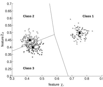
additional information, a reliable classification is almost unfeasible. At least one further feature is needed to extend the classifier´s input dimensions and to make a separation of the two different clusters, in the feature space, possible. The salient issue is how to get this additional feature? Figure 1 shows the two-dimensional feature space, with training examples, for an exemplary classification task of a fault detection system. Class 1 is referred to as the “normal” class, which means that input vectors belonging to this class indicate a normal process state. Class 2 and Class 3 are referred to as “abnormal” classes, which means that patterns belonging to one of these classes indicate an abnormal process state.
Figure 1: Feature space of an exemplary two-dimensional classification task of a
fault detection system with training patterns (patterns with Class 1 label ( ), patterns with Class 2 label ( ), patterns with Class 3 label ( )). The black dots mark cluster centers which, in this special case, correspond to the classificator’s prototype vectors of each class.
It is important for the fault detection system to not only classify an input vector according to the “normal” or “abnormal” classes but in case of an abnormal class, there needs to be a differentiation between the Class 2 and Class 3 types of faults. This is because the classification into Class 2 or Class 3 may have different consequences for the further process control. For example, Class 2 may indicate increased mechanical forces as a result of strong load alterations while Class 3 indicates increased mechanical forces due to attrition. The consequence of the classification of an input vector to Class 2 may warrant a logbook entry, while the classification of an input vector to Class 3 may require a recommendation for maintenance by the fault detection system. The three clusters shown in Figure 1
0.3 0.4 0.5 0.6 0.7 0.8 0.9
0.2 0.25 0.3 0.35 0.4 0.45 0.5 0.55 0.6 0.65 0.7
feature 1
fe
a
tu
re
2
Class 1 Class 2
Class 3
feature
have 2D Gaussian distributions with equal standard deviations 1 2 0 03. . The
positions for the mean values for each cluster are marked with the big black dots. In this case the cluster centers also correspond to the prototype vectors (sometimes also referred to as codebooks [2]), which are used to come to a classification decision, for any input vector based on the Euclidean metric and the nearest neighbor rule. The resultant decision borders, which yield a Voronoi tessellation, are shown as black lines. In this special case the decision borders even equal the optimal decision borders – the Bayesian borders [2]. From Figure 1 it can be clearly seen that a classification of an input vector into Class 2 or Class 3 may be uncertain as both cluster centers are very close to each other, and the clusters therefore overlap. However, if the transition speed from the normal class into the different abnormal classes has different values, the reliability of a classification into Class 2 or Class 3 could be improved by considering additional information regarding the temporal order of previous input vectors. The PID concept described below is a methodology to treat both previous and current input vectors to form additional PID values which then make the use of expert knowledge regarding the different transition speeds applicable for the decision-making.
The PID Concept
Especially in mechanical systems where monitoring and fault detection is applied, the appearance of fault signature input vectors are not arbitrary. When mechanical systems start to wear via creep, the representative input vectors will also change slowly. The spatial-temporal characteristics of these input vectors form a directed movement through the feature space, accompanied with the inevitable presence of noise. These slowly moving features due to mechanical wear can differentiate from those patterns which occur as a result of a sudden special event. One can thus use this expert-knowledge about the spatial-temporal movement of previous input vectors in order to classify a current input vector more reliably.
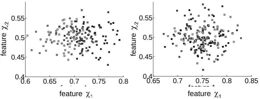
The two clusters shown in Figure 2 represent Gaussian distributed two-dimensional
data sets
X
x
k
2| k
1
,...,
200
. In the left cluster the mean value of feature1
is constantly decreasing, whereas the mean value of feature 2 is constant. In contrast, the right cluster shows a Gaussian distribution with constant mean values for both feature 1 and feature 2. Both clusters consist of 200 input vectors each.
Figure 2: Two-dimensional clusters which illustrate the grey scale colour coding to indicate the temporal order of appearance of the input vectors. As time progress the colour of the input vector spot becomes lighter Left: The mean value of feature 1 is constantly decreasing while the mean value of feature 2 is constant, which results
in a directed movement to the left. Right: The mean values of both features are constant.
To return to the classification problem shown in Figure 1, one can imagine that the clusters shown in Figure 2 are examples for input vectors belonging to Class 1 – the
“normal” class. As described earlier, the Class 2 points arise from increased mechanical forces as a result of strong load alterations while Class 3 points correspond to increased mechanical forces due to attrition. Due to the fact that mechanical attrition usually is a creeping process, a directed movement of previous input vectors into the direction of Class 2 and Class 3 in the feature space usually precedes those input vectors which belong to Class 3. The left cluster of Figure 2
indicates such a directed movement, whereas the right cluster does not. To express such chronological characteristics of previous input vectors mathematically, the PID concept calculates the distances between the prototype vector of the “normal” class
w1 and the current input vector xk for each of the n dimensions by
1
k k n n n
d
, (3)
the discrete-time integration of dnk
1 1
1 1
k
k i
k i k kn n n n n n
i i
d d d d , (4)
as well as the discrete-time derivative of dnk
1
1 1
1
k
k k k
kn n n n n n n
d
d
d
. (5)Beyond the nearest neighbor rule, which is only based on the prototype vectors and the current input vector, we now have three additional PID-values per dimension n:
0.6 0.65 0.7 0.75 0.8
0.4 0.45 0.5 0.55
feature 1
fe
a
tu
re
2
0.65 0.7 0.75 0.8 0.85
0.4 0.45 0.5 0.55
feature 1
fe
a
tu
re
2
feature feature
fe
a
tu
re
fe
a
tu
The P-value (3), the I-value (4) and the D-value(5). These PID-values can be integrated into the decision-making process to be able to come to a more reliable classification. Figure 3 and Figure 4 show different examples of an uncertain classification and illustrate the performance of the PID concept. Both Figures are based on the two-dimensional clustering problem as shown in Figure 1.
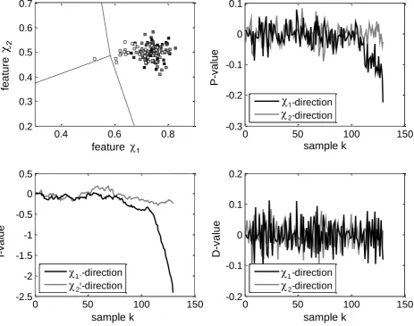
Figure 3: First example of an uncertain classification, where the spatial-temporal
appearances of previous input vectors form a visible directed movement. Top left: Scatter plot in the two-dimensional feature space. Top right: P-values calculated according to (3). Bottom left: I-values calculated according (4). Bottom right: D-value calculated according to (5).
In Figure 3 the 130th sample is assumed to be the current input vector which needs to be classified. Based on the nearest neighbor rule alone it would be classified to Class 2 as it can be seen from the scatter plot (Figure 3, top left). This classification is quite uncertain because this input vector is close to the decision boundary to Class 3. The spatial-temporal appearances for the 25 previous input vectors already show a directed movement into the direction of Class 2 and Class 3. Armed with this additional knowledge an expert would probably classify the 130th input vector to
0.4 0.6 0.8
0.2 0.3 0.4 0.5 0.6 0.7
0 50 100 150
-0.3 -0.2 -0.1 0 0.1 x1-direction x2-direction
0 50 100 150
-2.5 -2 -1.5 -1 -0.5 0 0.5 x1-direction x2-direction
0 50 100 150
Class 3 based on the knowledge that the directed movement indicates attrition rather than load alterations. Therefore the additional PID-values supplied by the calculations (3), (4) and (5) could be used to incorporate the expert knowledge into the decision making or to calculate a relevance factor for the current classification. As it can be seen from Figure 3 (bottom left) at k=130 the I-value in 1-direction is
reduced by about -2.4 due to the directed movement of previous input vectors. This is a distinctly lower value than the P-value in 1-direction at k=130, which is only about
-0.23 (Figure 3, top right). In contrast the D-value is constantly in a range about +/- 0.11 (Figure 3, bottom right). To illustrate the benefit of using these PID-values
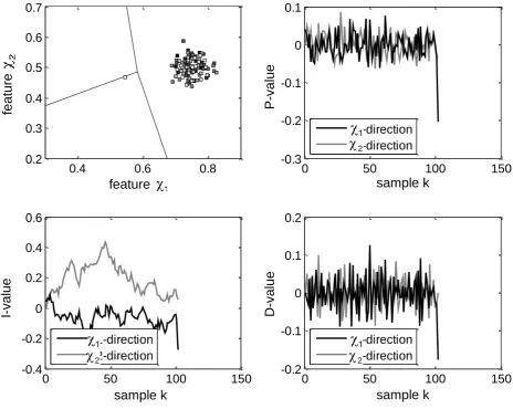
Figure 4 shows an example of a classification, where based on expert knowledge, a Class 2 classification is more appropriate.
Figure 4: Second example of an uncertain classification, where the spatial-temporal
appearances of previous input vectors do not form a visible directed movement.
Top left: Scatter plot in the two-dimensional feature space. Top right: P-values
calculated according to (3). Bottom left: I-values calculated according (4). Bottom
right: D-value calculated according to (5).
0.4 0.6 0.8
0.2 0.3 0.4 0.5 0.6 0.7
0 50 100 150
-0.3 -0.2 -0.1 0 0.1
x1-direction x2-direction
0 50 100 150
-0.4 -0.2 0 0.2 0.4 0.6
x1-direction x2-direction
0 50 100 150
-0.2 -0.1 0 0.1 0.2
x1-direction x2-direction
sample k
sample k sample k
feature
2
2
2
fe
a
tu
re
I-va
lue
P
-va
lue
D
-va
In Figure 4 the 101st sample is assumed to be the current input vector which needs to be classified. Based on the nearest neighbor rule alone this input vector would be classified to Class 3, although it is so close to the decision boundary that one might have the impression this input vector would even be on the decision boundary (Figure 4, top left). One can further see from the scatter plot that the 101st sample occurs far away from the previous ones. With this additional knowledge about previous input vectors, an expert would probably classify the 101st input vector to Class 2, as in this case there is not a directed recognizable movement in the spatial-temporal order of previous input vectors. Again the additional PID-values could be used to integrate this expert knowledge to the decision making process. As it can be seen from Figure 4 (bottom left) the I-values perform a random walk around 0, which certainly might peak to +/-0.5. At k=101 the I-value in 1-direction and the P-value in
1
-direction are about -0.26, and -0.2 respectively. The D-value, which in the previous example has never been lower than -0.11, has a value about -0.17 (Figure 4, bottom right). Table 1 summarizes the PID-values in 1-direction of the current input vectors for both examples.
Table 1: PID-values in 1-direction for the examples of Figure 3 and Figure 4
P-value in 1
-direction
I-value in 1
-direction
D-value in1
-direction
Example of Figure 3 -0.23 -2.4 -0.08
Example of Figure 4 -0.2 -0.26 -0.17
Examining Table 1 the modulus of the PID values are more or less equal for the example of Figure 4 indicating that there is no directed movement of previous input vectors. In contrast for the example of Figure 3 the PID values differ markedly i.e.
|I| > |P| > |D| a sign for directed movement.
Discussion
The PID concept is just a kind of data preprocessing that involve previous input vectors which already have been classified, in order to gather additional information for the classification of a current input vector. How to employ these additional features for a more reliable classification is up to the user’s discretion. A relevance factor can be calculated based on the PID-values which then gives information about the reliability of a current classification that is actually only based on the nearest neighbor rule. Another possibility is to directly use the PID-values as additional input dimensions and to thus expand the dimensions of the input space.
assumed to be deterministic, with the time sample points to be equidistant. If the time slot
1
k k k
T t t , (6)
is varying, where tk is the time that a current sample k occurs at, this needs to be
considered.
For a varying time slot, Equation (4) is modified to be
1
11 1
k
k i i
k i i k k kn n n n n n
i i
d T d T d d T , (7)
and Equation (5) is modified to be
1
1 1
1
k k k k
n n n n
k n n
n
k k
d d d
T T . (8)
For practical applications it should be noted that the prototype vectors rarely fits with the mean values of the class distribution, implying that in certain dimensions there is a normal distance between prototype values and mean values. For these dimensions the I-value then grows over time and might indicate a directed movement of the input vectors, which actually is not there. To eliminate this problem the moving average
1
1 1
k
kk i i
n n n n
i k c i k c
d d
c c , (9)
can be employed instead of the time-discrete integration dnk, where c is a filter
constant to be chosen according to the application using expert knowledge. Indeed the range of values the moving average (9) can have is limited, whereas that of the time-discrete integration (4) is not limited. This difference needs to be considered when applying (9) instead of (4) and subsequently interpreting the PID-values for pattern classification. In contrast to the time-discrete integration dnk which distinctly
indicates a directed movement with a high modulus >|P|, the moving average dnk is
only equally to the P-value in case of a directed movement.
Conclusions
In this paper we proposed a PID concept to give further information that can be used for the decision making in pattern classification tasks. The concept has been targeted to the special clustering problem, which is often encountered in fault detection systems, where due to sensor hardware limitations, abnormal process states cannot be properly classified as the clusters of these process states overlap in the feature space. However in fault detection, the fact that certain features often have different alteration rates when processes change from “normal” states to different “abnormal” states can be exploited. To make this expert knowledge usable, the PID concept calculates three additional values for each input dimension based on the distances between input vector and prototype vector of the “normal” class. In a practical application the discrete-time integration of the distance between an input vector dimension and a prototype vector dimension often results in an error as the mean value of the “normal” input vectors does not necessarily match with the normal prototype vector. Due to this fact the calculation of the moving average of the distance instead of its time-discrete integration is recommended.
Approaches for cases where a classification task has more than one “normal” class is not discussed in this paper, but will be the subject of our future work in this field.
References
[1] J. B. MacQueen: Some methods for classification and analysis of multivariate observations. Ft. Belvoir: Defense Technical Information Center, 1966.
[2] T. Kohonen: Self-organizing maps. Berlin, New York: Springer, 1995.
[3] D. Atherton: Control Engineering: An introduction with the use of Matlab: Ventus Publishing ApS, 2009.
[4] K. J. Åström and T. Hägglund: The future of PID control. Control engineering practice : CEP ; a journal of IFAC, the International Federation of Automatic Control, no. 11, pp. 1163–1176, 2001.
[5] O. Föllinger, F. Dörrscheidt, and M. Klittich: Regelungstechnik: Einführung in die Methoden und ihre Anwendung, 8th ed. Heidelberg: Hüthig, 1994.
[6] K. J. Åström and R. M. Murray: Feedback systems: An introduction for scientists and engineers. Princeton: Princeton University Press, 2008.
[7] A. E. Smith, D. W. Coit, and C. W. McCullers: Reliability Improvements of Airport Ground Transportation Vehicles Using Neural Networks to Anticipate System Failure. Proceedings of the Annual Reliability and Maintainability Symposium; International Symposium on Product Quality & Integrity; RAMS, Piscataway, NJ: IEEE Operations Center, 2002.