Scheduled Review Methods for Controllable State Variables

(1)

Scheduled Review Methods for Controllable

State Variables

H. Salehi Fathabadi

*

Department of Mathematics and Computer Science, University of Tehran, Tehran, Islamic Republic of Iran

Abstract

In many real systems in which a state variable should be controlled for being in

appropriate range, the length of control (review) intervals is taken to be constant.

In such systems, when the cost of reviews and out-of-range values of the state

variable are considerable, this method may not be optimal. In this paper we let the

length of review intervals to be variable during each operating cycle and construct

the related mathematical cost model. Then two scheduled review methods, called

U

2

and U

3

, are introduced and the relative annual system costs are analyzed. The

model is developed for the case of negative exponential variate as the time

between successive consumption points. It is shown that the new methods results

a significant reduction in the expected annual cost of the system.

Keywords: State variables; Inventory systems; Random variates; Review methods

* _{E-mail: [email protected]}

1. Introduction

In many real systems there exist critical state variables whose values must be kept within a predefined range. If they cross the range boundaries, a cost will be incurred. The nature of the state variables in such systems is stochastic so that it is not known (or computable) when it will reach its boundaries. Usually, in order to control a state variable in such system, the values of the variable are reviewed either continuously or periodically. Certainly, when reviews incur cost and take time they have to be performed discontinuously.

At a review time, if it is observed that the variable has crossed the borders, proper action is taken to adjust the value of the variable. Production and inventory systems, security systems inspection, soil moisture in agricultural activities and some of medical systems are well known examples of such systems.

A system whose annual cost model is considered in this paper consists of a state variable V, which, due to stochastic consumption, is always decreasing (except when its value is adjusted). It is assumed that the upper and lower boundaries are positive real number ω and ν, respectively. When, by a review, the value of V is observed to be equal to or less than νit is increased up to the level ω. The review and increment cost is fixed at A. In some systems, such as inventory systems, negative net values of V cause both constant and time dependent costs.

This kind of cost is called shortage or backlog cost. We assume that each negative unit of V during a time of length t incurs π +πˆt unit of cost. Of course holding positive values for V adds up to the system’s cost. Assume this cost is h for a positive unit of V for one unit of time.

(2)

to check whether V has reached or crossed ν. If it has not, the review would not have any effect except its cost. In most of the so far proposed review methods the inter-review times (periods) are taken to be equal and constant, see for example [1-3]. In order to decrease the overall shortage cost, Teunter et al. [6] suggested emergency reviews in addition to the regular reviews. In fact, the decreasing nature of V implies that the subsequent review intervals need not to be of the same length as the preceding ones. Salehi Fathabadi [4] introduced an inventory control policy in which the lengths of review periods are computed as a function of inventory level. Within this policy the total annual system cost will considerably decrease when shortage costs are high.

In this paper, first we construct a general annual cost model for variable review intervals. Three reviewing methods are described and applied to the general model. Then methods’ efficiency, when the time length between consumption points is negative exponential, are compared.

Through the paper we assume that the consumption time is stochastic and occurs in single unit; the intervals between successive consumption events are independent and identically distributed.

2. The General Cost Model

Let Xt be the consumption on V during a time

interval of length t with probability function p(x, t) and mean µt, where µ is the expected consuming rate. Let the time origin be defined as the instant of increasing the state variable up to ω. Also suppose Ur, r = 1, 2, 3,…

are the review times measured from the time origin and U0 = 0.

Now let Z be the time taken by the state variable to reach the level ν, starting from the time origin. If the p.d.f of Z is denoted by f (z) and its cumulative distribution function by F(z), then

1 0

( ) ( ; ) 1 ( ; )

m

x m x

F z p x z p x

∞ −

= =

=

∑

= −

∑

z

]

)

(2.1)

and f (z) =d F (z)/dz, where m=ω−ν.

Suppose the value of V is observed to be ν or less at a review time Ur, so that Ur−1<z≤Ur. The cycle length in

this case is Ur. Therefore, if the number of reviews

du-ring a cycle is denoted by R, its expected value will be

1 1

( ) [ ( _r) ( _r )

r

E R r F U F U

∞

− =

=

∑

− ,

and the expected cycle length is

1 1

[ _R] _r[ ( _r) ( _r )

r

E U U F U F U

∞

− =

=

∑

− . (2.2)

At any time t during a cycle, 0 < t ≤ Ur, the expected

net value of V is ω - µt and the expected shortage is 0 for t ≤ z and

( ) ( ; x ν

x v p x t z ∞

=

− −

∑

for t > z. Define V+_{= Max. {V, 0} and V}−_{= Max {}₋_V, 0}. Since V+_{= V + V}−_{the expected cost of holding} positive V, subjects to Ur−1 < z ≤ Ur is

1( ) [ ( )

( ) ( ; )

r

r u r

ο

u

ο

x ν

C U h ω μt dt

]

x v p x t z dt ∞

=

= −

+ − −

∫

∑

∫

(2.3)

Assuming π +πˆt as the cost of one unit of V−_{for a} time interval of length t, the conditional expected cost of shortage in a cycle is

2( ) ( ) ( , )

ˆ r ( ) ( ; )

r r

x ν

u

ο

x ν

C U π x ν p x U z

π x v p x t z dt

∞

=

∞

=

= − −

+ − −

∑

∫

.

) (2.4)

Therefore the expected total cost of operating the system per cycle. E[CR], is

1

1 1

2

1 2

1

[ ] [ ( )

( )] ( )

[ ]

[ ( ) ( )] ( ) .

r

r U

R r

U r

r

U

r r

U r

E C A rJ C U

C U f z dz

A JE R

C U C U f z dz

−

∞

=

∞

=

= + +

+

= +

+ +

∑∫

(2.5)

where J is the cost of one review. We use E[CR]/E[UR]

as a measure of the expected total annual cost. Let

ˆ

( ) Ur ( ) ( ; )

z x ν

h π x v p x t z dt ∞

=

+

∫

∑

− −

( ) ( ; x ν

π x v p x t z ∞

=

+

∑

− −

(3)

simplification of (2.5) gives the expected annual cost of the system as:

1 2 1 ( , , ) { [ ] [ ] 1 [ ] 2 ( , ) ( ) } / [ ] r r R R U r U r R

K ν ωU A JE R hωE U

μhE U g U z f z dz

E U − ∞ = = + + − +

∑∫

(2.6)

In general case we assume the consumption

distribution provides for existence of and

where F’ (.) = 1 − F (.). It is easy to see that ( )

0F U r

r ∞ ∑ =

( )

0rF U r

r ∞ ∑ = 0 0

[ ] ( ) lim ( )

( ), r n n r r r

E R F U nF U

F U ∞ →∞ = ∞ = ′ ′ = − ′ =

∑

(2.7)

According to the above assumption E[R] exists. Now consider that

2

ˆ

( , ) ( ) ( ) ( )

ˆ

1/ 2( )

r U r

z

g U z h π μ t z dt πμ U z

h π μβ πμβ

= + − + −

= + +

∫

r

)

where β = Ur − z. For non-increasing series of {Ur −

Ur−1}r = 1,

1 1 2 1 1 1 1 1 1 ( , ) ( ) ˆ

[1/ 2( )( )

( )] (

ˆ

[1/ 2( ) ]

r r r r U r U r r r r U r r U

g U z f z dz

μ h π U U

πU U f z dz

μ h πU π U

− ∞ = ∞ − = − ₋ ≤ + − + − ≤ + +

∑∫

∑

∫

Thus 1 1 ( , ) ( ) r r U r U r

g U z f z dz

−

∞

=

∑∫

is finite. Also if

only the first n terms of this summation are summed up, the error will be

1 1 2 1 1 ( , ) ( ) ˆ

[1/ 2( )( )

( )] ( ) r r U n r U r n n n

n n n

e g U z f

μ h π U U

πU U F U

− ∞ = + + + = ≤ + − ′ + −

∑ ∫

z dz

(2.8)

Since F’ (Un) → 0 as n→∞ and (Un+1− Un) ≤ U1, en

tends to 0 as n→∞. Hence en can be made as small as

desired.

3. Review Methods

In the classical treatment of the discrete review policy [2], as stated earlier, the length of all review intervals are taken as equal. In many cases such policy represents an easy schedule and implementation from a practical point of view. But the increasing hazard rate function, f (z)/[1−F(z)], of Z provides for succeeding review intervals shorter than the preceding ones. We consider two other simple methods for generating review times. In the first method the length of the first period is different from the later periods. In the second one the first two periods differ from the others. The classical review method is also included in the analyzing of the cost function and comparison.

3.1. Periodic Review Method, U1

In this method review times are generated as: , 1, 2,3,

r

U =rT r = _K (3.1)

Let U1 denotes the set of times generated by this

method. We have

1 0 0 [ ] [ ( ) ( ) [ ] ( ), R r r r r

E U T r F U F U

TE R

T F U ∞ − = ∞ = ′ ′ = − = ′ =

∑

] r r (3.2) and

2 2 2

1 1

2

0 0

[ ] [ ( ) ( )]

[2 ( ) + ( )],

R r

r

r r

E U T r F U F U

T rF U F U

∞ − = ∞ ∞ = = ′ ′ = − ′ ′ =

∑

(3.3)

since, the existence of _{( )} implies that n2_F’ 0rF U r

(4)

(Un)→0 as n→∞. Hence E [UR] and E [UR2] exist and

the cost function can be calculated to any level of accuracy.

3.2. One Period Scheduled Review Method, U2

In this method, apart from the first review in a cycle, the reviews are periodic. Let the length of the first review period be denoted by T1 and the length of the

subsequent periods be denoted by T. Thus review times, U2, are generated by:

1 ( 1) , 1, 2, r

U =T + −r T r = _K (3.4)

It is obvious that T1 is not less then T, so that {Ur−

Ur−1} r=1 is non-increasing. Using the convergence

assumption of ( ) and we have

0F U r

r ∞ ∑

= r 0rF U r( )

∞ ∑ =

1 1

1

1 1

[ ] [ ( 1) ][ ( ) ( )

( )

R r

r

r r

E U T r T F U F U

T T F U

∞

− =

∞

=

′ ′

= + − −

′ = +

∑

]

r

(3.5)

This is convergent to a finite time length. Also it is easy to see that.

2 2 2

1

0

1 1

[ ] 2 ( )

(2 ) ( )

R r

r

r r

E U T T rF U

T T T F U

∞

=

∞

= ′

= +

′

+ −

∑

(3.6)

3.3. Two Periods Scheduled Review Method, U3

In this method the first two review intervals are different in length from the subsequent intervals. The review times, U3, are scheduled as:

1 1 1 2

,

( 2) , 2,3, 4, r

U T

U T T r T r

=

= + + − = _K (3.7)

Obviously T1≥ T2≥ T and, within this method, {Ur−

Ur−1} r−1 is also non-increasing. In this method, with a

simple formulation we get

1 2 1

2

[ _R] ( ) (

r

E U T T F T T F U

∞

= ′

= + +

∑

′ _r) (3.8)

and

2 2

1 2 1 2 1

1 2

2 2

2

[ ] (2 ) ( )

(2 2 3 ) ( )

2 ( )

R

r r

E U T T T T F T

T T T T F U

T rF U ∞

=

∞

=

′

= + +

′

+ + −

′ +

∑

(3.9)

4. Negative Exponential Consumption Intervals

We suppose that the intervals between successive occurrence of consumption have negative exponential density function. That is,

( ) λt, 0

g t =λe− t > . (4.1)

This gives

( , ) ( )x λt / !, 0,1, 2,

p x t = λt λe− x x = _K (4.2) and

1

( )

( 1)! m m λz

λ z e f z

m − −

=

− , (4.3)

This shows that Z is a Gamma variate. Since, for this probability function,

1

lim ( 1) / ( )

lim ( 1) ( ) /[ ( )]

r r

r

r r

λt

F U F U

r F U rF U

e →∞

+ →∞

−

r

′ + ′

′ ′

= +

=

(4.4)

for all the three methods, and

exist, and therefore the assumptions about these terms are valid.

( )

0F U r

r ∞ ∑

= r 0rF U r( )

∞ ∑ =

4.1. Numerical Evaluation of Optimal Decision Variables

For numerical determination of optimal decision variables, ν, ω, T1, T2 and T, either a numerical method

capable of handling non-linear functions, mixed integer and real variables has to be exploited, or an iterative procedure is applied. To apply the latter approach an upper bound on m has to be established.

First Euler-Maclaur summation formula, is used to find exact or nearly exact values of E[UR] and E[U2R]

(5)

0 0 (1) (1) (3) (3) (2 1) 2 (2 1) 1

Φ( ) Φ( ) (Φ( ) Φ(0)) 2

(Φ ( ) Φ (0)) /12

(Φ ( ) Φ (0)) / 720

(Φ ( )

Φ (0)) / 2 ! .

n _n r k k k k

r x dx n

n n B n k B = − − = + + + − − − + + − +

∑

∫

L (4.5)

where Bk’s are Bernoulli numbers and Φ(j) (.) is the jth

derivative of Φ(.) and Rk is the remainder which is

smaller, in absolute value, than the first neglected term. Denoting (4.3) by fm (z), taking σ1 = T1− T, σ2 = T2 +

T1− 2T and using (4.5) we get the following results for

the three review methods: (i) – For U1 and m>3:

[ ] /( ) 1/ 2

E R =m λT + (4.6)

[ _R] / / 2

E U =m λ+T (4.7)

2 2

[ _R] ( 1) / /

E U =m m+ λ +mT λ+T3 ₃_(4.8)

(ii) – For U2:

1 1

[ ] 1 ( ) /( )

( / 1/ 2) ( ) ( ) /12 m

m m

E R mF σ λT

T T F σ Tf σ

+

′ = +

′

− − + ₁

1)

)

12

(4.9)

1 1 1 1

2

1 1

[ ] ( ) / (

( )/2 ( ) /12

R m m

m m

E U T mF σ λ σ F σ

TF σ T f σ

+

′ ′

= + −

′

− + (4.10)

2 2

2 1 2

1 1 1

2 2

1 1

2

1 1 1

[ ] ( 1) ( ) /

( ) /

( / 3) (

( ) ( ) /

R m

m

E U m m F σ λ

mTF σ λ T

T T F σ

T T σ f σ

+ + ′ = + ′ + + ′ − − + + (4.11)

(iii) – For U3:

1 2

2 2

2

[ ] 1 ( ) /( )

( / 1/ 2) ( ) ( )

( ) ( ) /12

m

m m

E R mF σ λT

σ T F σ F σ

F σ T Tf σ

+ ′ = + ′ ′ − + + ′ − + 2 2 (4.12)

1 2 1

2 2 1 2

2

2 2

[ ] ( )

( / 2 ) ( ) ( ) /

( ) ( ) /12

R m

m m

E U T T F T

T σ F σ F σ λ

TF σ T T f σ

+ ′ = + ′ ′ − + + ′ − + (4.13) 2 2

1 2 1 2 1

2 2 2 2 2 2 2 2 2 2 2 2 1 2

[ ] (2 ) ( )

(2 / 3 ) ( )

(2 3 ) ( )

( 2 ) ( )

( 1) ( ) /

( ) / R m m m m m m

E U T T T T F T

T σ F σ

Tσ T F T σ

T T σ f σ

m m F σ λ

mTF σ λ

+ + ′ = + + ′ − + ′ − + + + + ′ + + ′ + (4.14)

It should be reminded that the error in the use of (4.9) to (4.14) is very small for moderately large m. In order to get an upper bound for m, the value of

1

1 ( , ) ( )

r

r U

r

r U− g U z f z dz

∞

=

∑ ∫ must be found for at least

large values of m.

Theorem 1. In the review methods U1, U2 and U3

1 1

lim r ( , ) ( ) ( ) /

r U

r m

r U

r

g U z f z dz G T T

−

∞

→∞

∑∫

₌ = (4.15)

where

0

1 _ˆ

( ) { [2 ( ) ] ( 1; )

2

ˆ

( 1)( ) ( 1; ) /(2 )

ˆ

[ ( ) ] ( ; )} . T

G T λy π h π y P ν y

ν ν h π P ν y λ ν π h π y Pν y dy

= + +

+ + + +

− + +

∫

−

and

P

(K, y) is the complementary cumulative

distribution of poison variate.

Proof. The proof is for the three review method separately. First consider that by using

( ) ( ; ) ( ) ( 1;

( ; )

x ν

x ν p x t z λ t z P ν t z

νP ν t z ∞ = ) − − = − − − − −

∑

and 1 0 1

( ; ) ( ; ) /( 1)

( )! ( 1; ) /[ ( 1)( 1)

T

n n

n

t P ν t dt T P ν T n

ν n P n ν T λ n ν

+ + = + − + + + + −

∫

!]

(6)

0( ) 1₂ [2 ( ˆ) ] ( 1; )

ˆ

( 1)( ) ( 1; ) /(2 )

ˆ

[ ( ) ] ( ; )

g β λβ π h π β P ν β ν ν h π P ν β λ ν n h π β P ν β

= + + −

+ + + −

− + +

(4.16)

(a) Ur = r T, r = 1, 2, 3. Let n be an integer satisfying n

− 1 < (m − 1)/ λT ≤ n for m > 1, and n = 1 for m = 1. Let

α =Min. {fm (Un−1), fm (Un)}. Since g0 (β) ≥ 0,

1 0 1 1 1 1 ( ) ( ) ( )[ ( ) ( ) ( ) r r U m U r m r r

m n m n

g β f z dz

G T f U

f U f U α

− ∞ = ∞ − = − ≥ − +

∑∫

∑

] + (4.17)

Using (4.5), for m>1 we get

1

( ) 1/

m r

r

f U T

∞ = =

∑

, Thus 1 0 1 1 ( ) ( ) ( ) / ( )[ ( ) ( ) ] r r U m U r

m n m n

g β f z dz G T T

G T f U f U α

− ∞ = − ≥ − +

∑∫

− (4.18) Also 1 0 1 1 ( ) ( ) 1 ( )[ ( ) ( )] 1 ( ) / ( ) ( ) r r U m U r

m r m

r

m

g β f dz

m

G T f U f

λ

m G T T G T f

λ − ∞ = ∞ = − ≤ + − = +

∑∫

∑

(4.19)

Since fm (U n), fm (Un−1) and fm ((m − 1)/λ) tends to

zero as m→∞, the proof in this case is completed. (b) Ur = T1 + (r − 1) T, r = 1, 2, 3…. In this case

suppose m > λT1 + 1 and n satisfies T1 + (n − 2) T < (m

− 1)/λ≤ T1 + (n − 1) T. Then in a similar way we get

1 0 1 1

1 2 ( ) ( ) ( ) ( ) 1 ( )[ ( ) ( )]. r r u m m u r

m r m

r

g β f z dz G T f T

m

G T f U f

λ − ∞ = ∞ = ≤ − + +

∑∫

∑

Applying Euler’s formula, we have

1 1 1

2

( ) ( ) / 1/ 2 ( ) ( ) Re

m r m m m

r

f U F δ T f δ f T

∞ = ′ = − −

∑

+ . where

1 1 1

| Re |≤λT f[ m−( )δ −fm( )]δ . Therefore

1 0 1

1

1 1

1 1 1

( )

( ) ( ) ( )

1

( ) ( ) ( )[ ( )

1/ 2 ( ) ( )

( ) /12 ( ) /12] r r u m m u r m m m m m m G T g β f z dz F δ

T

m G T f T G T f

λ

f δ f T

λT f δ λT f δ

− ∞ = − ′ ≤ − + + − − + −

∑∫

(4.20) Similarly

1 0 1

1

1 1

( )

( ) ( ) ( )

( )[ ( ) /12 ( ) /12

1/ 2 ( ) ( ) ( ) ]

r r u m m u r m m

m m u m n

G T g β f z dz F δ

T

G T λT f δ λT f δ

f δ f U f U α

− ∞ = − − ′ ≥ + − − − − +

∑∫

1 (4.21)

where α is defined as in case (a). Note that

1 1

1 δ f_m(m ) F_m( )δ₁ 1

λ

− _′

− ≤ ≤ (4.22)

and lim F’ (δ1) = 1 when m→∞. Canceling all terms

inside the square brackets in (4.20) and (4.21), when m→∞, proves Theorem in this case.

(c) U1 = T1, Ur = T1 + T2 + (r − 2)T, r = 1, 2, 3. In this

case, by taking m >λ (T1 + T2) + 1 and n satisfying T1 +

T2 + (n − 3) T < (m − 1)/λ ≤ T1 + T2 + (n − 2)T the

proof is similar to case (b).

To establish the upper bound on m, first consider the U1 method. Let for a precision factor, ε, M1 be such an

integer that if m > M1 then the absolute difference

between

1 0

1 ( ) ( )

r

r u

m r u− g β f z dz

∞

=

∑ ∫ and G (T)/T is less than

ε. Let M = Max. {3, M1}. For m > M the cost function

(7)

1

2 2 2

2

( , , ) /

2

/ 3 2

2 ( )

(2 )

λA

K ν ωU J ω

m λT m m λT h

m λT

λG T T m λT

= + +

+ − − +

+

T h

(4.23)

By taking m as a continuous variable and solving

∂K/∂m =0, we have

1 2

0 2

1 [2 ( ( )) /( ) /12

/ 2] 1/ 2

m λ AT G T hT λT

λT λT

= + −

+ −

2

1 +

(4.24)

Now an upper bound on m can be taken as:

0 1( ) Max.{3, 1,[ ] 1}

m T = M m (4.25)

in which [x] is the greatest integer less than or equal to x.

In the case of U2 and U3, let M2 and M3 be the

counterparts of M1 with the corresponding T.

Considering (4.9) to (4.11) in case of U2, it is not

difficult to see that if m > M2 then

1

[ ] [ _R]/ /

E R =E U T −δ T (4.26)

[ _R] / / 2

E U =m λ+T (4.27)

and

2 2

[ _R] ( 1) / / /

E U =m m+ λ +mT λ+T 2 ₃_(4.28)

Also using (4.12)-(4.14), we see that if m > M3 then

E[R], E [UR] and E [UR2] for U3 have the same values as

(4.26)-(4.28) respectively with δ1 substituted by δ2.

Finally the annual cost function in case of U2 and U3

methods becomes

3 2 2

1

2

( , , ) /

2

/ 3 2

2 [ ( ) ]

(2 )

i

λA

K ν ωU J ω

m λT m mλT h

m λT

λG T Jδ

T m λT −

= + +

+

− +

+ − +

+

T h

(4.29)

Taking the same approach as in the case of U1

method, the upper bound for m in U2 method will be

0 2( , ) Max.{1 2,[ 2] 1}

m T T = M m + (4.30)

where

1 2 0

2 2 2

[2 ( ( ) )/( )

/12 / 2] 1/ 2 .

m λ AT G T Jδ₁ hT

λT λT λT

= + −

− + −

(4.31)

In the case of U3, m03 is the same as (4.31) with δ1

replaced by δ2 and the upper bound on m is

0 2( , , ) Max.{1 2 3,[ 3] 1}

m T T T = M m + (4.32)

4.2. Model Optimization

As it is seen, minimization of the annual cost function is very complicated. It is a mixed integer and real optimization problem for which no known method exists. Therefore a heuristic method has to be applied.

Being able to determine an upper bound for m we suggest the following iterative search procedure to evaluate the optimal values of the related decision variables.

1. Guess values for T, T1, and T2 as appropriate.

2. Guess ν.

3. Evaluate m1 (T), m2 (T1, T) or m3 (T1, T2, T) as

appropriate.

4. Find ω0 in the interval (ν, mi + ν) which gives the

lowest cost function value.

5. Fixing ω to ω0 find ν0 which gives the lowest cost

function value.

6. If ν0 is different from ν, set ν = ν0 and start from

step 3.

7. Using ω0 and ν0, find the related optimal value of

T, T1, and T2 as appropriate.

8. If the predefined accuracy level on interval lengths has been reached stop otherwise start from step 3.

In general for given values of ν and ω, the annual cost function has several minima in terms of the review intervals. This creates the possibility that a normal search procedure terminates with a local solution. Figures 1, 2 and 3 illustrate this point.

Further numerical investigations suggest that K is unimodal with respect to T in both U2 and U3 when T1

(and T2) are fixed. Furthermore when T is set to its

optimal value, then K is unimodal with respect to T1 in

both of the methods (see Figs. 4 and 5).

The above remarks suggest that if steps 7 and 8 in the search procedure are replaced by the following steps then the results are very likely to be global. Given an initial value of T1 (E[z] for example):

1. Minimize K with respect to T. Denote the best value found for T as T0.

2. Set T = T0 and search for the best value of T1 and

denote it by T1, 0.

(8)

step 1.

The optimal values of T1 and T are found when two

consecutive values of T or T1 are equal.

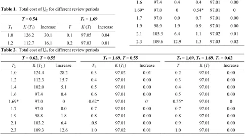
In the investigation on review periods, it has been observed that T1 is the most effective period in U2 and

U3. For example, in case U2, T1 causes a significant

variation in K (T1) when T is optimal. In contrast, for

optimal T1, K (T) is rather a flat function. Tables 1 and

2 demonstrate the effect of the first review periods on the annual cost function in the cases of U2 and U3.

80 130 180 230 280 330

0 1 2 3 4 5

Review period, T

K(

T

)

Figure 1. Total cost of U1 method.

80 81 82 83 84 85 86 87 88 89 90 91

0 1 2 3 4 5 6

First review period, T1

K(

T

1

)

50 60 70 80 90 100 110

0 1 2 3 4 5 6

K(

T

1

)

Figure 5. Total cost of U3 for optimal T2 and T3.

60 70 80 90 100 110 120 130 140 150 160

0 2 4 6 8 10

K(

T

1

)

40 60 80 100 120 140 160

0 2 4 6 8 1

K(

T

1

)

0

(9)

Table 1. Total cost of U2 for different review periods

T = 0.54 T1 = 1.69

T1 K (T1) Increase T K (T) Increase

1.0 126.2 30.1 0.1 97.05 0.04

1.2 112.7 16.1 0.2 97.03 0.01

1.4 102.0 5.2 0.3 97.02 0.00

1.6 97.4 0.4 0.4 97.01 0.00

1.69* 97.0 0 0.54* 97.01 0

1.7 97.0 0.0 0.7 97.01 0.00

1.9 98.9 1.9 0.9 97.01 0.00

2.1 103.3 6.4 1.1 97.02 0.01

2.3 109.6 12.9 1.3 97.03 0.02

Table 2. Total cost of U3 for different review periods

T = 0.62, T = 0.55 T2 = 1.69, T = 0.55 T2 = 1.69, T2 = 1.69, T1 = 0.62

T2 K (T2 ) Increase T1 K (T1) Increase T K (T) Increase

1.0 124.4 28.2 0.3 97.02 0.01 0.2 97.01 0.00

1.2 112.3 15.7 0.4 97.01 0.00 0.3 97.01 0.00

1.4 102.0 5.1 0.5 97.01 0.00 0.4 97.01 0.00

1.6 97.4 0.4 0.6 97.01 0.00 0.5 97.01 0.00

1.69* 97.0 0 0.62* 97.01 0′ 0.55* 97.01 0

1.7 97.0 0.0 0.7 97.01 0.00 0.7 97.01 0.00

1.9 98.8 1.8 0.8 97.01 0.00 0.8 97.01 0.00

2.1 103.2 6.4 .0.9 97.01 0.00 0.9 97.01 0.00

2.3 109.3 12.6 1.0 97.02 0.01 1.0 97.01 0.00

Table 3. Minimum total annual cost of U1 (top entry) and U2

πλ

8 10 20 30 40 100

29.7 33.7 50.4 64.0 76.1 132.2

1 29.7 33.7 50.4 64.0 76.1 132.1

45.3 50.9 73.1 89.8 104.3 166.7

9 44.5 50.1 71.9 88.4 102.9 162.8

54.3 64.0 89.5 108.7 124.0 197.2

99 58.8 60.5 83.4 100.7 115.3 182.0

Table 4. Minimum total annual cost for U1 (top entry) and U2

πλ _{8 10 20 40}₁₀₀

29.7 33.7 50.4 76.1 132.2 1.5 29.7 33.7 50.4 76.1 132.1 40.5 44.9 62.9 89.0 141.9 10 39.5 44.2 62.2 88.4 141.6 50.9 55.3 75.8 103.3 161.4 100 48.9 53.2 73.5 101.1 157.5

Table 5. Minimum total annual cost of U2 (top entry) and U3

πλ _{8 10 30}₁₀₀

44.5 50.1 88.4 162.8

9 44.4 50.1 88.4 161.7

54.8 60.5 100.7 182.0

99 54.7 60.5 100.7 181.8

5. Comparison of the Review Methods

Considering the three review methods, the minimum total annual cost is used for comparing their performa-nce. Table 3 compares U1 with U2 for different values of λ and π. In this comparison ν and ω have been set to their optimal values. We see that there is no practical difference for small π (relative to h) and low value of λ. For large π and λ, U2 is a more desirable method.

Table 4 also compares U1 with U2 for different

values of π and λ. Here we observe that the difference is not much, even for large values of ˆπ and λ.

Table 5 demonstrates that the extra complication of U3 does not yield considerable improvement with

respect to U2.

6. Conclusion

Generally, in a consideration of different review times, the periodic review method should be compared with U2. There is no great practical and computational

(10)

References

1. Chuang B.R., Ouyang L.Y., and Chuang K.W. A note on periodic review inventory model with controllable setup cost and lead time. Computers and Operations Research,

31(4): 549-561 (2004).

2. Freeland J.R. and Porteus E. Evaluating the effectiveness of a new method for computing approximately optimal (s, S) inventory policies. Operations Research, 28: 353-364

(1980).

3. Roundy R.O. and Muckstadt J.A. Heuristic computation of periodic-review base stock inventory policies.

Management Science, 46(1): 104-109 (2000).

4. Salehi Fathabadi H. Dynamic review periods in the (s, S) inventory control policy. J. Science, University of Tehran,

22(1): 37-42 (1996).

5. Shahani A.K. and Munford A.G. A nearly optimal inspection policy. Operational Research Q, 23: 373-379

(1972).

6. Ruud T. and Dimitrios V. An inventory system with periodic regular review and flexible emergency review.