Determining suitable model for zoning drinking water distribution network based on corrosion potential in Sanandaj City, Iran

Determining suitable model for zoning drinking water distribution

network based on corrosion potential in Sanandaj City, Iran

Parvin Dehghani Parvin Dehghani Parvin Dehghani Parvin Dehghani1111

, , ,

, BehzadBehzadBehzadBehzad _{ShahmoradiShahmoradiShahmoradiShahmoradi}1111

, Ata Amini , Ata Amini , Ata Amini , Ata Amini2222

, Mohammad Sedigh Sabeti , Mohammad Sedigh Sabeti , Mohammad Sedigh Sabeti , Mohammad Sedigh Sabeti3333

1 Kurdistan Environmental Health Research Center, Kurdistan University of Medical Sciences Sanandaj, Iran 2 Agricultural and Natural Resources Research Center of Kurdistan, Sanandaj, Iran

3 Department of Civil Engineering, School of Technology, Islamic Azad University, Sanandaj Branch, Sanandaj, Iran

Abstract Abstract Abstract Abstract

Corrosion in general is a complex interaction between water and metal surfaces and materials in which the water is stored or transported. Water quality monitoring in terms of corrosion and scaling is crucial, and a key element of preventive maintenance, given the economic and health hurts caused by corrosion and scaling in water utilities. The aim of this study is to determine the best model for zoning and interpolation corrosive potential of water distribution networks. For this purpose, 61 points of Sanandaj, Iran, distribution network were sampled and using Langelier indices, we investigated corrosivity potential of drinking water. Then, we used geostatistical methods such as ordinary kriging (OK), global polynomial interpolation, local polynomial interpolation, radius-based function, and inverse distance weighted for interpolation, zoning and quality mapping. Variogram analysis of variables was performed to select appropriate models. The results of the calculation of the Langelier index represented scaling potential of drinking water. Suitable model for fitness on exponential variogram was selected based on less (residual sums of squares) and high (R2_{) value. Moreover, the best method for interpolation was selected using the}

mean error and root mean square error. Comparison of the results indicated that OK was the most suitable method for drinking water quality zoning.

KEYWORDS: KEYWORDS: KEYWORDS:

KEYWORDS: Water Quality, Inverse Distance weighted, Kriging, Radius-Based Function, Zoning, Interpolation, Corrosivity, Sanandaj

Date of Date of Date of

Date of submission:submission:submission:submission:27 Oct 2013, Date of acceptance:Date of acceptance: 13 Jan 2014Date of acceptance:Date of acceptance:

Citation: Dehghani P, Shahmoradi B, Amini A, Sabeti MS. Determining suitable model for zoning drinking

water distribution network based on corrosion potential in Sanandaj City, Iran. J Adv Environ Health Res

2014; 2(2): 72-80.

Introduction

Drinking water must be void of any mixtures that may be harmful to human health. Most of the developing countries suffer from hygienic problems resulting from lack of drinking water and absence good quality and microbiological

contamination.1 _{It is estimated that}

approximately 5 million children die annually due to inappropriate drinking water quality.2

Corresponding Author Corresponding AuthorCorresponding Author Corresponding Author::::

Behzad Shahmoradi

Email: [email protected]

One of the qualitative parameters in water distribution network is corrosion. Corrosion is one of the most complicated and costly problems facing drinking water utilities.3 _{Corrosion can}

affect public health, public acceptance of water supply and the cost of providing safe drinking water. Corrosion in drinking water distribution system causes lots of hygienic and economic problems, for instance, internal corrosion causes pipe fractures, overflowing, pipe obstruction, quality change and odor, color and taste production. Rapid urban development brings

about more demand and vaster development of water network system. More complexity of the water network, the more data processing. For data processing and management, systems with easier access and faster functioning are needed.4

Determining optimized zoning method and quality model of drinking water can be a fundamental step in quality data management of water in the district. Geographical information systems (GIS) have effective usage in managing geo-spatial information and qualitative and quantitative information.5 _{In such a situation, the}

interpolation of data points is the most suitable

option that can handle the spatial

characteristics.6 _{Spatial interpolation models}

include geographical location of sample data points.7 _{Some spatial interpolation models for}

creating qualitative model of drinking water include distance-reverse weighting inverse distance weighted (IDW), spline, Kriging and polynomial interpolation, among which ordinary Kriging (OK) and IDW are widely used.8 _Earls

and Dixon compared interpolation models for IDW spline and data rainfall spatial Kriging using ArcGIS software (version 9.3, Esri, Redlands, CA, USA). She found that Kriging models (Kriging-exponential) produce better results than IDW and spline models.9 _Naoum

and Tsanis rated spatial interpolation according to the decision-making systems based on GIS. They found that OK (Kriging-exponential)

produce reliable estimates.10 _Evaluating

geostatistical methods like Kriging, radius-based function (RBF), local estimating, and global estimating, Shaabani found that Kriging models are better tools to analyze salinity and nitrate of underground water due to their lower root mean

square error (RMSE) and higher R2.11

Taghizadeh Mehrjardi et al. studied spatial

evaluation of qualitative parameters of

underground water like TDS, TH, EC, SAR, SQ4,

Cl− _{according to IDW, Kriging and co-Kriging}

models; their results show that Kriging model is better based on RMES criterion.12 _Kriging

modeling nitrate pollution of underground

water resulting from agricultural activities, Piccini et al. showed that it is a suitable method for identifying vulnerable areas from nitrate perspective.13 _{The same findings were reported}

by other researchers.14-17 _{Ghaneian et al.}

investigated corrosion and precipitation potential in Dual water distribution system in Kharanagh District of Yazd Province and determined that water had precipitative quality.18 _{Dehghani et al.}

used Langelier saturation index (LSI) for corrosion zoning of water distribution system in Shiraz, Iran. Regular monitoring and analyzing water samples, they found that scaling potential in water samples was high.19 _{The aim of the}

present study is to zone the corrosion potential of drinking water distribution network of Sanandaj, Iran, using LSI and the most appropriate interpolation and variogram models in GIS.

Materials and Methods

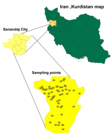
Sanandaj, the capital of Kurdistan province, covering an area of 3688.8 ha is located in the western part of Iran and the southern part of the province. Its geographical coordination is latitude N 14 35´ and longitude E 46 (Figure 1). Its height differs from 1450 to 1538 m above sea level. It is also located in the mountainous region of Zagros and has cold and semi-arid weather. Its average temperature is 15.20, 25.20, 10.40, and 1.60 °C in spring, summer, autumn, and winter respectively. The maximum temperature in July is 44 and the minimum temperature in February is −13.5 °C.

In this study, we collected water samples randomly from 61 points of the drinking water distribution network of Sanandaj. Latitude and longitude of the samples location was recorded via GPS. Each water sample was tested for corrosion perspective according to the standard methods for water and wastewater examination.20 _{LSI was used}

to determine the corrosion potential of drinking water. It is based on pH of the water sample.21

LSI was determined using Equation. 1. LSI=pH-pHs (1)

Equation. 2.

Figure 1. Location and sampling points of study area

pHs = (9.3+A+B)-(C+D) (2) Where, A = (Log10 [TDS]-1)/10 = 0.15;

B = −13.12 × Log10 (°C + 273) + 34.55 = 2.09 at 25° C and 1.09 at 82° C;

C = Log10 (Ca2+ _{as CaCO3)−0.4 = 1.78, (Ca}2+ _as

CaCO3 is also called calcium hardness and is

calculated as = 2.5(Ca2+_);

D = Log10 (alkalinity as CaCO3) = 1.53

For LSI > 0, water is supersaturated and tends to precipitate a scale layer of CaCO3, whereas, for

LSI = 0, water is saturated (in equilibrium) with CaCO3. A scale layer of CaCO3 is neither

precipitated nor dissolved. For LSI < 0, water is under saturated and tends to dissolve solid CaCO3.

If the actual pH of the water is below the calculated saturation pH, the LSI is negative, and the water has a very limited scaling potential. If the actual pH exceeds PHS, the LSI is positive

and being supersaturated with CaCO3, the water

has a tendency to form scale. At increasing positive index values, the scaling potential increases. In practice, water with an LSI between −0.5 and +0.5 will not display enhanced mineral dissolving or scale forming properties. Water

with an LSI below −0.5 tends to exhibit noticeably increased dissolving abilities while water with an LSI above +0.5 tends to exhibit noticeably increased scale forming properties.

Data were analyzed according to descriptive statistics. Average, variance, standard deviation, maximum and minimum, skewness and kurtosis were calculated using SPSS for Windows (version 16.0, SPSS Inc., Chicago, IL, USA). Among various deterministic interpolation techniques OK, global polynomial interpolation (GPI), LPI, RBF and IDW were used for determining the best interpolation method. For this reason, Arc GIS 9.3 and GS+ (version 5.1, Gamma Design Software, Plainwell, MI, USA) were used. Full explanation of geostatistical methods could be found in the literature.11,12,17,22-24 _{In general, geostatistical}

analyzing is based on this theory that measuring with smaller distances is more likely to be similar that with more distances (this means that the local coefficient exists). This theory can be verified using semivariogram examination that is an appropriate tool for measuring the coefficient among samples. Semivariogram is calculated using Eq. 3.25,26

( )

i i

i=1

1

γ

h

[ (x )-Z(x +h)]

2N(h)

Z

=

∑

(3) Where, N (h) is the number of observation pairs separated by distance h, Z (xi) is the value

of the variable Z at the xi location and (xi + h) is

the value of the variable Z at xi + h location.

Therefore, a graph is created for each variable that variance between points showed that during the modeling process of a semivariogram, the suggestions for cross-validation model are considered as a function of distance. In cross-validation method, an observational point is eliminated in each stage, and it is estimated based on other observational points. There would be a point estimated for each observational point. This method was used for verification. Variogram is composed of Nugget effect (C0), sill (C + C0) and range effect (A0). The

sample-taking or data analyzing. By the increase of h, the semivariogram modifies increases till it reaches a specific value. Then, it becomes constant. This distance is called the Range effect, and the value of the constant semivariogram modify is called the sill that is the spatial variance of the being studied variable. The experimental semivariogram γ (h) is fitted to a theoretical model such as linear to sill, gaussian, spherical, linear and exponential. Cross-validation was conducted in order to verify the accuracy and precision of the process. The model with the highest R2 _{and the lowest residual sums}

of squares (RSS) was selected. Nugget/sill in geostatistics can be considered as a criterion for spatial dependence. OK, GPI, local polynomial interpolation (LPI), RBF, and IDW were used for interpolation and predicting variance error of the non-sampling place.

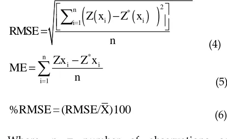
Finally, we evaluated the model function in cross-validation using below criterion. For determining the best interpolation method, three criteria of RMSE, mean error (ME) and %RMSE were used that are computed using Eq. 4-6.17

( )

( )

(

)

n *

i i

i=1

Z x

Z x

RMSE

n













=

∑

−

(4)

* n

i i

i=1

Zx

Z x

ME

n

−

=

∑

(5)

RMSE

%RMS

E = (

/X

)100

Where, n = number of observations or samples; Z*(xi) = observed values; Z(xi) =

predicted or estimated values, X = mean of measured parameter; and ME is the ME indication bias. Positive values of ME show

values more than real and negative values show estimates less than real. The more ME is smaller, the less the interpolation is skewed. RMSE values in the optimized state (the state in which the estimated and measured values are equal) is zero. The more RMSE is smaller, the more the estimating of interpolation method is accurate.27

RMSE is sensitive to wide values. Therefore, RMSE% can be used. This criterion being small is a reason for more accurate estimates, i.e., less difference between the real and estimated values. The accepted %RMSE value is 40 and values more than 70 show imprecision in the estimated points and high difference between the real and estimated values.28

Results and Discussion

A result relating to data’s being normal after normalizing the data, we examined it using statistical Kolmogorov-Smirnov test in SPSS 16 software. Table 1 presents a statistical summary of the corrosion situation of the drinking water distribution network of Sanandaj. The data were

distributed normally according to the

Kolmogorov-Smirnov test, skewness, and

histogram (Figure 2). Data normalization is a criterion only for Kriging methods.

Analysis of LSI variogram

GS+ software was used to create a semi-variogram for each variant and choosing the best theoretical corrosion model. Variogram is a useful plot by which many information could be extracted including data spatial structures,

radius correlations of variants, static

examination of data, and variant isotropic. Less RSS and more R2 _{were used for fitting the best}

model on the variogram and stronger spatial structure. Nugget/sill (C0/C0+C) ratio in the

geostatistics can be regarded as a criterion to classify the spatial dependence of quality parameters of water. If this ratio is <25%, the

Table 1. Results of statistical analysis on Langelier saturation index

N Minimum Maximum Mean Std. Skewness Kurtosis

Figure 2. Data histogram of Langelier saturation index

variant owns strong spatial correlations. If the ratio is between 25% and 75% the spatial correlations is medium. And if the ratio is more than 75% the spatial correlations are weak.25

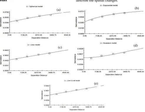
Figure 3 shows the variogram of the measured Langelier indices. Moreover, table 2 tabulates the results of the best models of exponential, linear, spherical and Gaussian linear to sill variants for the measured indices. Nugget /Sill ratio is between 0.4 and 0.7 indicating medium spatial coefficient. Based on the criteria of higher R2 _{and less RSS, exponential variogram}

is the best-fitted model. It has the strongest spatial correlations and Gaussian has the weakest.10,11,15 _{This model was also used to}

describe the spatial changes.

Figure 3. Fitted variogram models of Langelier saturation index (a) spherical, (b) exponential, (c) linear, (d) Gaussian, (e) linear to sill

(a) (b)

(c) (d)

Table 2. Best-fitted variogram models of Langelier saturation index

Model Nugget Sill Range Effective Proportion R2 RSS

C0 C0 + C Parameter A0 Range A1 C0/(C0 + C)

Spherical 0.04130 0.08370 6642 6642 0.507 0.974 8.47E-06 Spherical 0.03900 0.07910 2397 7191 0.507 0.998 7.72E-06 Linear 0.04221 0.06934 3234.4388 3234.4388 0.3910 0.961 1.301E-03 Linear to sill 0.04240 0.11800 9099 13130 0.641 0.961 1.13E-04 Gaussion 0.04770 0.10540 4608 7981.2901 0.547 0.890 3.18E-04 C0: Nugget effect; C + C0: Sill; A0: Range effect; R2: Regression coefficient; RSS: Residual sums of squares

Comparison of geostatistical methods

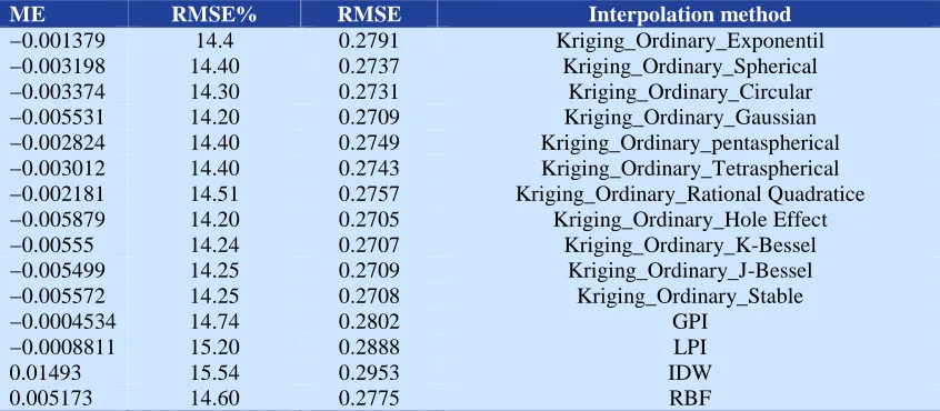
For determining the best interpolation method between the methods of geostatistical OK, GPI, LPI, RBF, IDW criteria of RMSE, ME, and %RMSE were used. As table 3 indicates, the value of ME and %RMSE in OK is less than others. The value of < 15 for %RMSE shows very

good accuracy of semi-variogram in

estimations.26 _{The OK model is the best for}

zoning. Zoning results of this paper is consistent to those of Naoum and Tsanis,10 _{Earls and}

Dixon,9 _{and Goovaerts.}29 _{Langlier saturation}

index zoning is shown by OK, GPI, LPI, RBF, and IDW maps (Figure 4). Langlier index has more sediment potential in North West, South East and central parts. Sediment is not balanced. It is strong in some parts and weak in other parts. Compared with North West and South East parts, central parts have weak sediment

potential. Few parts of North East, South West and West have weak corrosion potential.

Conclusion

Deterioration of materials resulting from corrosion can necessitate a colossal annual expenditure of scarce resources for repairs replacement and maintenance of distribution system. Given results obtained of drinking water in the Sanandaj distribution network has the scale formation potential. OK estimates with an exponential variogram based on RMSE and ME criteria is the most suitable technique for mapping quality spatial changes of LSI and assess the probability of exceeding the critical threshold. The advantage of krigingcompared with other methods is that kriging produces better estimates than the other methods because the method takes explicit account of the effects

Table 3. Selection of the most suitable model for evaluation on variogram

ME RMSE% RMSE Interpolation method

−0.001379 14.4 0.2791 Kriging_Ordinary_Exponentil −0.003198 14.40 0.2737 Kriging_Ordinary_Spherical −0.003374 14.30 0.2731 Kriging_Ordinary_Circular −0.005531 14.20 0.2709 Kriging_Ordinary_Gaussian −0.002824 14.40 0.2749 Kriging_Ordinary_pentaspherical −0.003012 14.40 0.2743 Kriging_Ordinary_Tetraspherical −0.002181 14.51 0.2757 Kriging_Ordinary_Rational Quadratice −0.005879 14.20 0.2705 Kriging_Ordinary_Hole Effect

−0.00555 14.24 0.2707 Kriging_Ordinary_K-Bessel

−0.005499 14.25 0.2709 Kriging_Ordinary_J-Bessel

−0.005572 14.25 0.2708 Kriging_Ordinary_Stable

−0.0004534 14.74 0.2802 GPI

−0.0008811 15.20 0.2888 LPI

0.01493 15.54 0.2953 IDW

0.005173 14.60 0.2775 RBF

Figure 4. Spatial variations maps of Langelier saturation index by interpolation methods of OK, GPI, LPI, RBF, and IDW

of random noise and identifies the optimal interpolation weights and searches radius and provides an indication of the reliability of the estimates. Kriging analysis leads to an increased understanding of the data sets obtained for the fouling potential. The accuracy of the kriging map not only depends on the variogram and the maximum number of samples or neighboring points in kriging, but also depends on the number of classes and class boundaries. LSI calculations and plotted zoning maps revealed that the chemical quality of drinking water distribution network in Sanandaj City is imbalanced; hence, causing scale formation in water distribution network systems, and other facilities are unavoidable. Moreover, health and economic outcomes, consumers dissatisfaction due to quality changes, loss of water pressure in the distribution network are another potential drawbacks of this issue. Finally, it is suggested that the concerned authorities take crucial and required measures to make the water more stabilized from the corrosion point of view before delivering it to the customers. Moreover, analyzing other physicochemical parameters is essential in giving better figure of the water quality in the studied area.

Conflict of Interests

Acknowledgements

The authors would like to thank Deputy of Research, Kurdistan University of Medical Sciences, Sanandaj, Iran for financial supporting this research work. The results presented in this paper is a part of M. Tech Dissertation of the first author.

References

1. van Leeuwen FX. Safe drinking water: the toxicologist's approach. Food Chem Toxicol 2000; 38(1 Suppl): S51-S58.

2. Wadud A, Chouduri AU. Microbial safety assessment of municipal water and incidence of multi-drug

resistant Proteus isolates in Rajshahi, Bangladesh. Current Research in Microbiology and Biotechnology 2013; 1(4): 189-95.

3. Sander A, Berghult B, Ahlberg E, Broo AE, Johansson EL, Hedberg T. Iron corrosion in drinking water distribution systems-Surface complexation aspects. Corrosion Science 1997; 39(1): 77-93.

4. Dawoud MA, Darwish MM, El-Kady MM. GIS-Based Groundwater Management Model for Western Nile Delta. Water Resour Manage 2005; 19(5): 585-604. 5. Tabesh M, Saber H. A Prioritization Model for

Rehabilitation of Water Distribution Networks Using GIS. Water Resour Manage 2012; 26(1): 225-41. 6. Cressie N, Wikle CK. Statistics for Spatio-Temporal

Data. New Jersey, NJ: John Wiley & Sons; 2011. 7. Maselli F, Chiesi M. Evaluation of statistical methods

to estimate forest volume in a mediterranean region. Geoscience and Remote Sensing 2006; 44(8): 2239-50. 8. Zimmerman D, Pavlik C, Ruggles A, Armstrong M. An

Experimental Comparison of Ordinary and Universal Kriging and Inverse Distance Weighting. Mathematical Geology 1999; 31(4): 375-90.

9. Earls J, Dixon B. Spatial interpolation of rainfall data using ArcGIS: A comparative study. Proceedings of the 27th Annual ESRI International User Conference; 2007 Jun 18-22; San Diego, CA.

10.Naoum S, Tsanis K. Ranking spatial interpolation techniques using a GIS-based DSS. Global Nest: the Int J 2004; 6(1): 1-20.

11. Shaabani M. Evaluation Geostatistical methods for mapping of groundwater quality and their zoning Case Study: Neyriz Plain, Fars Province. Journal of Natural Geography Lar 2011; 4(13): 93-6. [In Persian]. 12.Taghizadeh Mehrjardi R, Mahmoodi Sh, Heidari A,

Sarmadian F. Application of geostastical methods for mapping groundwater quality in Azarbayjan Province, Iran. Am Eurasian J Agric Environ Sci 2008; 3: 726-35. 13.Piccini C, Marchetti A, Farina R, Francaviglia R.

Application of Indicator kriging to Evaluate the Probability of Exceeding Nitrate Contamination Thresholds. International Journal of Environmental Research 2012; 6(4): 853.

14.Hooshmand A, Delghandi M, Izadi A, Aali A. Application of kriging and cokriging in spatial estimation of groundwater quality parameters. African Journal of Agricultural Research 2011; 6(14): 3402-8. 15. Maqami Y, Ghazavi R, Abbasali V, Sharafi S.

Evaluation of spatial interpolation methods for water quality zoning using GIS Case study, Abadeh Township. Geography and Environmental Planning 2011; 22(2): 171-82.

Basin/Jordan. Research Journal of Environmental and Earth Sciences 2012; 4(2): 177-85.

17.Li J, Heap AD. A review of comparative studies of spatial interpolation methods in environmental sciences: Performance and impact factors. Ecological Informatics 2011; 6(3-4): 228-41.

18.Ghaneian MT, Ehrampoush MH, Ghanizadeh GH, Amrollahi M. Survey of corrosion and precipitation potential in dual water distribution system in kharanagh district of yazd province. Toloo-E-Behdasht 2008; 7(3-4): 65-72.

19.Dehghani M, Tex F, Zamanian Z. Assessment of the potential of scale formation and corrosivity of tap water resources and the network distribution system in Shiraz, South Iran. Pak J Biol Sci 2010; 13(2): 88-92. 20.Clesceri LS, Eaton AD, Greenberg AE. Standard

Methods for the Examination of Water and Wastewater. Washington, D.C: American Public Health Association; 1998.

21.Kumar P, Sanand VS, Santhosh Kumar N, Sreerama Murthy B. Assessment of water quality of thatipudi reservoir of vizianagaram district of andhra pradesh. Innovare Journal of Science 2013; 1(2): 20-4.

22.Samanta S, Pal D, Lohar D, Pal B. Interpolation of climate variables and temperature modeling. Theor Appl Climatol 2012; 107(1-2): 35-45.

23.Rawat KS, Mishra AK, Sehgal VK. Identification of Geospatial Variability of Flouride Contamination in Ground Water of Mathura District, Uttar Pradesh, India. Journal of Applied and Natural Science 2012; 4(1): 117-22.

24.Babak O, Deutsch C. Statistical approach to inverse distance interpolation. Stoch Environ Res Risk Assess 2009; 23(5): 543-53.

25.Shi J, Wang H, Xu J, Wu J, Liu X, Zhu H, et al. Spatial distribution of heavy metals in soils: a case study of Changxing, China. Environ Geol 2007; 52(1): 1-10. 26.Hengl T, Heuvelink GBM, Stein A. A generic framework

for spatial prediction of soil variables based on regression-kriging. Geoderma 2004; 120(1-2): 75-93.

27.Mishra U, Lala R, Liuc D, Van Meirvenned M. Predicting the Spatial Variation of the Soil Organic Carbon Pool at a Regional Scale. Soil Science Society of America Journal 01/2010; 74(3) 2010; 74(3): 906-14.

28.Flipo N, Jeannee N, Poulin M, Even S, Ledoux E. Assessment of nitrate pollution in the Grand Morin aquifers (France): combined use of geostatistics and physically based modeling. Environ Pollut 2007; 146(1): 241-56.