Object Recognition based on Local Steering Kernel and SVM

(1)

International Journal of Engineering

J o u r n a l H o m e p a g e : w w w . i j e . i r

Object Recognition based on Local Steering Kernel and SVM

R. AhilaPriyadharshini*, S. Arivazhagan

Department of Electronics & Communication Engineering, Mepco Schlenk Engineering College, Sivakasi, Tamil Nadu, India

P A P E R I N F O

Paper history: Received 25 August 2012

Recivede in revised form 22 January 2013 Accepted 16 May 2013

Keywords: Object Recognition Salient Point Detector Patch Extraction Local Steering Kernel Principal Component Analysis

A B S T R A C T

The proposed method is to recognize objects based on application of Local Steering Kernels (LSK) as Descriptors to the image patches. In order to represent the local properties of the images, patch is to be extracted where the variations occur in an image. To find the interest point, Wavelet based Salient Point detector is used. Then, Local Steering Kernel is applied to the resultant pixels in order to obtain the most promising features. The features extracted will be over complete; so, in order to reduce dimensionality, Principal Component Analysis (PCA) is applied. Further, the sparse histogram is taken over the PCA output. The classifier used here is Support Vector Machine (SVM) Classifier. Bench mark database used is UIUC car database and the results obtained are satisfactory. The results obtained using LSK kernel is compared by varying parameters such as patch size, number of salient points/patches, smoothing parameter and scaling parameter.

doi:10.5829/idosi.ije.2013.26.11b.03

1. INTRODUCTION1

Natural resources which are not limited to any size and which show arbitrarily complex scenes, are classified according to whether they contain a certain object or not, this is Generic Object Recognition [1]. Visual systems have ability to distinguish objects effectively. In the same way, machine vision systems must also perform and recognize objects at any position, size, and appearance. Generic object recognition systems do not include any information about specific objects rather they learn to recognize objects by inspecting training images and train the model and also recognize objects in unseen images [2]. Then, this model is used to recognize objects in unseen images. For each of the training images, a set of features are derived. Each feature describes properties of either the whole image (global feature) or a part of the image (local feature). Usually, local features are most successful in capturing the content of complex images.

To reliably recognize objects under varying circumstances (for example, objects appearing at different scales, rotation and translation) the features must be chosen in such a way that they are invariant with respect to these aspects. From the features of the

*_{Corresponding Author Email:} _{[email protected]} _{(R. Ahila}

Priyadharshini)

training images, the parameters of an underlying statistical model are estimated. Using these features and the trained model, the object recognition system outputs whether the trained object is contained in the image or not. Once trained, the performance of object recognition system is measured on a set of test images. The recognition rate on this set denotes the ratio of correctly classified images to all images in the test data set.

In complex images, the information provided by the global features is not sufficient and they are not well suited in this context. Hence, local features like patches are better suited for complex images, because they represent restricted regions of the image [1]. Beneficial properties of local features are inherent translation invariance, robustness to object variance and occlusion and possible scale invariance.

The reviews of the existing approaches for various submodules are discussed in the following:

Salient Point Detection: Global features describe

(2)

proposed by Haralick and Shapiro [3] are: Distinctness, Invariance, Stability, Uniqueness and Interpretability. Earliest method for interest point detector is Harris Corner Detector, but this seems to be rotationally invariant but not Scale invariant [4]. Though there are numerous interest point detectors Wavelet Based Salient Point extraction seems to be the best approach [5].

Features (LSK): Features such as histograms,

gradients and shape descriptors are all shown rapid growth in object recognition but the proposed method is based on the computation of the Local Steering Kernels as the descriptors which are local weights computed directly from the patch values themselves [6]. The advantages of this method are they use geodesic distance to measure the self-similarity of the pixels; LSK uses the radiometric and geometric pixel differences in computation of the kernel, robustness to noise and illumination changes. Quantization and informative feature selection on the features with little discriminative power decrease performance. Hence, densely computed LSKs are dimensionally reduced by using Principal Component Analysis to enhance the discriminative power and reduce the computational complexity [7]. After that, sparse histogram is applied to get bins as the features. Finally, the features are fed into support vector machine in order to classify.

In previous work of Takeda [8], basic kernel regression and steering kernel concepts have been discussed and the effectiveness of these kernels for applications such as Denoising and Interpolation are analyzed. Hae Jong Seo and Peyman Milanfar [6] proposed the use of Local Steering Kernel to measure the similarity of pixels for object detection, generic detection algorithm for Face verification using Localy Adaptive regression Kernels (LARK) [9], bottom up saliency detection algorithm to automatically detect salient objects in natural images [10].

Classification (SVM): An approach to object

Classification was proposed by Deselaers et al [11], where generative/discriminative object Classification using local features was done by the fusion of SVMs and Gaussian Mixture Densities. A comparison of learning and classifying techniques, such as, nearest neighbor methods, support vector machines, and convolutional networks is given by LeCun& Huang [12]. These techniques are studied for challenging conditions: complex images with high amount of “clutter”, varying pose, and lighting. In [13], the authors proposed amodified version of the fast global k-means (fast GKM) clustering method for clustering the gene expression datasets and Classification accuracy of SVM, Naïve Bayes, and KNN classifiers in gene expression datasets are compared. Mutch and Lowe [14] investigated the role of sparsity and localized features in a biologically-inspired model of visual object

classification and the classifier used is SVM. The error rate obtained is 0.06% in UIUC database. In this work, the Local Steering Kernels are used as descriptors and they are efficiently stored in sparse histogram and classified using SVM classifier.

In the previous work, local steering kernel is used for Object Detection, Image Denoising and Image Reconstruction; but, in this work it is used for Object Recognition. Here, the features extracted from LSK are represented by sparse histogram. The problem in normal histograms is that they become difficult to handle if the dimensionality of the input data is large, because the number of bins in a histogram grows exponentially with the number of dimensions of the data [15]. Thus, a sparse representation of the histograms is used, i.e., only those bins whose content is not empty are stored. The advantage of going for sparse representation is that the time taken for training and testing is very less compared to normal histogram approaches. The proposed method allows for recognizing objects under varying circumstances and shows excellent results in UIUC database.

The paper is structured as follows. The next section discusses the outline of the proposed method. In Section 3, Salient point detection, in particular the advantages of using wavelets for salient point detection are discussed. Section 4 deals with Feature Extraction such as Patch extraction and the computation of LSK over the patches and Section 5 deals with the steps involved in reducing the dimension of patches. Section 6 deals the representation of Sparse Histograms. Section 7 gives the recognition results for single scale (SS) and multi-scale (MS) images in UIUC Database. Finally, section 8 gives the conclusion of the proposed method.

2. OUTLINE OF THE PROPOSED METHOD

The first step is to detect the salient points using salient point detector. The interest points are formed in the region of high variance. The patches are extracted around each of these salient points. The preserved patches are manipulated by computing Local Steering Kernel over them and turned into feature vector where PCA dimensionality reduction is applied to extract the appropriate feature from the patches. Then, they are represented efficiently using sparse histogram. The histograms of the test and training images are compared using SVM classifier and classified.

3. SALIENT POINT DETECTION

(3)

local ones [5]. The aim is to find a relevant point to represent this global variation by looking at wavelet coefficients at finer resolutions. The algorithm for detecting relevant salient points using Haar wavelet transform is given as follows:

Ø Calculate the wavelet representation of an image for all scales j=1/2,…, 2-Jmax_{and spatial orientations}

d=1, 2, 3, where Jmax= log2[min(m, n)], m and n are

the width and height of an image.

Ø For each wavelet coefficient, find the maximum child coefficient.

Ø Track it recursively in finer resolutions.

Ø At the finer resolution (½), set the saliency value of the tracked pixel: the sum of the wavelet coefficients tracked.

Ø Choose the most prominent points based on the saliency value.

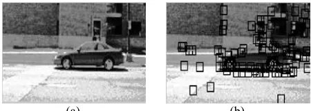
The tracked point and its saliency value are computed for every wavelet coefficient. A point related to a global variation has a high saliency value, since the coarse wavelet coefficients contribute to it. A finer variation also leads to an extracted point, but with a lower saliency value. Then, it is needed to threshold the saliency value, in relation to the desired number of salient points. The reason for choosing Haar wavelet transform is that it has compact support and simplest one. With the Haar wavelet, each coefficient is computed with 2-j _{signal points. Each point is used only} once, the spatial supports of these wavelets are not overlapping at a given scale. Figure 1 shows the result of salient point extraction.

4. FEATURE EXTRACTION

4. 1. Patch Extraction Objects of interest have

little contribution to global properties as they occupy only a part of the image, so Local descriptors are used. Patches are squared sub images extracted from the image over the Salient points [1]. The advantages of patches are (i) Reduction of the amount of data to be processed, (ii) Robustness to background clutter and (iii) Robustness to occlusion, variability in object shape.

Patch sizes play a vital role in the performance of the algorithm. Here, various patch sizes such as 7×7, 9×9 and 11×11 are selected for analyzing the performance of the Proposed Method. The result of Patch Extraction is shown in Figure 2.

4. 2. Local Steering Kernel (LSK) Local Steering

Kernel measures the Local similarity of pixel to its neighbor both geometrically and radiometrically. The key idea is to obtain Local data structures by analyzing the pixel difference based on estimated Gradients [8]. The LSK is modeled as Equation (1):

þ ý ü î

í

ì -

-=

- 2 ₂ 2

) ( ) ( exp 2

) det( ) (

h x x C x x h

C x

x

K l l T l l

l _p (1)

where, _l_Î

{

1,...._p2

}

,

xl=[x1,x2]T is the spatial coordunates, p2

is the number of pixels in a local window (p×p), h is a global smoothing parameter, and the matrix Cl is a

covariance matrix estimated from the collection of Gradient vectors [x1 ,x2]within the local window around

the sampling position x [7].

LSK captures data exceedingly well even in the presence of distortions, even in complex regions and in regions with mediocre levels of noise. The features extracted from LSK are stable in the presence of noises and robustness to illumination changes.The covariance matrix can be interpreted as averaging geodesic distances in a patch to obtain a robust estimation even in the presence of noise and other perturbations. The geodesic distance (xl-x)TCl (xl-x) is normalized to a unit

vector (i.e., a unit norm) to be more robust to illumination changes. In our work, LSK is applied to the gradient computed patches, not directly to image pixels; so this leads to enhanced feature vectors and the recognition obtained is high. For various patch sizes, the LSK is computed and by varying the smoothing parameter value h, the recognition rate is obtained.

5. FEATURE REDUCTION

For an n×n patch, there are n2_{dimensional feature}

vectors. Thus, dimensionality reduction of feature vector is desirable. A commonly used reduction method is principal component analysis (PCA).

(a) (b)

Figure 1. (a) Sample Car Image of UIUC database; (b) Salient

Points Extracted Image

(a) (b)

(4)

5. 1. Principal Component Analysis Principal component analysis is a method that reduces data dimensionality by performing a covariance analysis between factors [17]. PCA is an unsupervised approach to extract the appropriate features from the patches. It is used to lower the dimensionality of a data set with minimal information loss. PCA chooses a new coordinate system with the first axis pointing in direction of the greatest variance in the dataset; accordingly for second, third, etc. axis. By eliminating axis with a low variance, the dimensionality is reduced but only little information is lost mathematically.This is done by Eigen vector decomposition of the covariance matrix of the data set.

Descriptors obtained will be highly informative but when taken together tend to be over complete. Hence, dimensionality reduction step is applied to retain only the salient characteristics of Local Steering kernel [6]. The steps involved in PCA transformation are,

Ø For each patch compute mean vector µ and covariance matrix ξ.

Ø Find the Eigen values and Eigen vectors and sort them according to decreasing Eigen values.

Ø Retain the topmost m values as the Principal Components for that patch.

Here, various number of PCA coefficients such as 4, 6 and 8 are chosen and the performance evaluation is done. The values of PCA coefficients are varied in a large manner and are getting varied for different patches. In order to represent them in a well defined manner, sparse histogram is required.

6. SPARSE HISTOGRAM

Histograms are a well-known method to represent the distribution of data and are applied in field of computer vision [15]. A histogram H is a discrete approximation of the distribution of a random variable. It contains an array (H1, H2 ….HN) of bins representing a partition of the feature space S into N regions {S1…SN}. The regions

are usually of equal size, although it is not required. The number of bins N in H is vd_where_d_{is the}

dimensionality of the feature space S and v denotes the number of different values for each dimension. The problem when deriving histograms from image patches is that patches contain a high number of dimensions. If 20 dimensional PCA transformed patches were used, a histogram of these patches would contain v20_{bins. Even} with the smallest possible value for v of value 2, this result in 220 bins, which is not feasible [15]. Therefore, it is clear that the number of dimensions has to be reduced. To be able to deal with histograms of that size, a special sparse data structure is needed, because the explicit representation of all bins as an array is too memory consuming. Instead, a sparse representation storing only those bins which are not empty is used.

Using a membership function, an efficient access to the bins is possible. Due to the sparse representation of the histograms, they are called as “sparse histograms”. Ø For all patches of all training images, let xl= (xl1…

xlD) be the l-th PCA transformed patch with D

coefficients.

Ø (µ1 … µD) denotes the mean vector and (σ1 … σD) the

variance vector of all xl.

Ø Each patch x=(x1,………… xD) is assigned a “dimension value vector” S=(s1,……… sD) as in

Equation (2)

ï ï î ï ï í ì

+

-+ >

-<

=

otherwise :

2

)) x

)( 1 v (( round

x : 1 v

x : 0

S

d

d d d

as

as m as m

as m

(2)

where, d=1,2,…D; v is the number of different possible values per dimension and “round (…)” rounds a real number towards the nearest integer. Here, the value of v is chosen as 4.

Finally, q assigns each patch a corresponding histogram bin by uniquely mapping the dimension value vector onto the bins, numbered from 0 to vD_-1_{. The}

mapping function is given in Equation (3):

å

=

-= D

1 d

1 d dV

S

q ₍₃₎

Crucial parameter for choosing the membership function is α, which determines which part of S is to be represented by histogram. Thus, the recognition rates for various values of α such as 0.5, 1 and 1.5 are determined and the optimal parameter value is found. The bins are now used as features and fed into Classifiers. The classifier used here is OSU SVM Classifier Matlab Toolbox version 3.00 [18]. SVM is a type of learning machine, based on statistical learning theory, which uses Polynomial Classifiers, Neural Networks, and Radial Basis Function Kernel (RBF) networks as a special form. Here, non linear SVM classifier is used and suitable kernel used to convert the nonlinear domain into linear domain is RBF Kernel.

7. RESULTS AND DISCUSSIONS

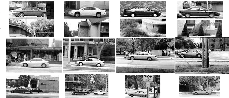
The proposed method is evaluated using the UIUC Database12. It contains 1050 training images (550 car and 500 non-car images) and 170 single-scale test images as well as 108 multi-scale test images. The training images are quite small (100×40) and quite roughly quantized, the test images are a bit bigger and may contain several cars. All images are in gray scale. They are of different resolutions and include instances

(5)

of partially occluded cars, cars that have low contrast with the background, and images with highly textured backgrounds. The sample images of UIUC database is shown in Figure 3.

7. 1. Performance Comparison of LSK Computed

Patch Over Simple Image Patch Table 1 shows the

recognition rate for images in UIUC car database without and with computing LSK over the patches of size 7×7. The recognition rate is high for the LSK computation. Figure 4 shows the ROC curves for the Single Scale and Multi Scale test images in the UIUC Database with and without computation of LSK. In order to determine the equal error rate, 170 negative images that do not contain the object category are considered.

7. 2. Optimal Parameters Veriication The

experiment is performed on both single-scale (SS) and Multi-scale (MS) test images by varying parameters such as patch size, number of salient points/patches extracted, smoothing parameter of LSK, scaling parameter of sparse histogram and number of PCA components.

7. 2. 1. Patch Size Patches of different sizes are

extracted around the region of interest. In [7], 9×9 patch size is used. Here, in addition 7×7, 11×11patches are also used. For each and every patch sizes, smoothing parameter, scaling parameter and number of PCA coefficients are varied and the results are analyzed.

7. 2. 2. Varying Smoothing Parameter Table 2

Shows the Recognition Rates for varying patch sizes and number of salient points/patches for various

Smoothing parameter values. Scaling parameter value used here is α=0.5. Number of PCA coefficients used here is 6. In [10] Smoothing parameter value used is 0.008. In [7], h=2.1 is used . Hence, in our framework three different values of h=0.008, 1, 2.1 are used. From the Table 2 it is inferred that patches of size 7×7 and 9×9 show better performance for all the parameter changes and seems to yield full recognition rate. The 11×11patch shows low recognition rates when compared to other patch sizes and for 150 salient points, 11×11 patch gives better results. For this work, h=1 gives better results irrespective of increasing the patch size and the number of patches extracted.

7. 2. 3. Varying Scaling Parameter Table 3 shows

the Recognition Rates for varying patch sizes and varying number of salient points/patches for various Scaling Parameter values (α). The choice of α varies from task to task. Here, the value of α is varied as 0.5, 1 and 1.5. Smoothing parameter value used here is h=1. In this case also patch size of 7×7 gives full recognition rate independent of the number of salient points and also the scaling parameter values for both Single and Multi scale test images.

TABLE 1. Comparison of recognition rates and ROC Equal

error rates for single scale (SS) and multi scale (MS) test images with and without LSK.

Patch Size (7×7) Recognition Rate (%) ROC EER (%)

SS MS SS MS

Patch+PCA 98.8 93.52 5.3 8.3

Patch+LSK+PCA 100 100 0 0

a

b

c

d

Figure 3. Sample images of UIUC database (a) Positive Training Images (b) Negative Training Images (c) Single Scale Test

(6)

Figure 4. ROC curves for the Single Scale and Multi Scale test images in the UIUC Database

TABLE 2. Recognition Rates in % by varying Smoothing Parameter value for various patch sizes and number of salient points for

Single Scale (SS) and Multi Scale (MS) test images

PATCH SIZES

RECOGNITION RATES (%)

Smoothing parameter h=0.008 Smoothing Parameter h=1 Smoothing Parameter h=2.1

No. of Salient points/Patches extracted No. of Salient points/Patches extracted No. of Salient points/Patches extracted

100 125 150 100 125 150 100 125 150

SS MS SS MS SS MS SS MS SS MS SS MS SS MS SS MS SS MS

7×7 100 100 100 100 100 100 100 100 100 100 100 100 100 100 100 100 100 100

9×9 100 100 100 100 100 100 100 100 100 100 100 100 100 100 100 100 100 100

11×11 96.47 99.07 99.4 100 99.4 100 97.64 99.07 99.4 100 100 100 88.23 97.2 97.6 100 98.23 100

TABLE 3. Recognition Rates in % by varying the Scaling Parameter

PATCH SIZES

Scaling parameter α=0.5 Scaling Parameter α=1 Scaling Parameter α=1.5

100 125 150 100 125 150 100 125 150

7×7 100 100 100 100 100 100 100 100 100 100 100 100 100 100 100 100 100 100

9×9 100 100 100 100 100 100 98.8 100 100 100 100 100 100 100 100 100 100 100

11×11 99.4 100 99.8 100 100 100 87.05 96.29 92.9 98.1 93.5 99.1 96.47 99.07 99.41 100 99.4 100

TABLE 4. Recognition Rates in % by varying the number of PCA coefficients

PATCH SIZES

Number of PCA coefficients=4 Number of PCA coefficients=6 Number of PCA coefficients=8

100 125 150 100 125 150 100 125 150

7×7 100 100 100 100 100 100 100 100 100 100 100 100 100 100 100 100 100 100

9×9 100 100 100 100 100 100 98.8 100 100 100 100 100 97.64 98.14 100 100 100 100

11×11 100 100 99.4 100 100 100 96.4 99.07 99.4 100 99.4 100 82.94 95.37 87.5 95.37 97.5 100

0 0.1 0.2 0.3 0.4 0.5 0.6 0.7 0.8 0.9 1

False positive rate

T

rue

p

os

iti

ve

r

ate

ROC curve for uiuc car singlescale

PCA LSK+PCA

0 0.1 0.2 0.3 0.4 0.5 0.6 0.7 0.8 0.9 1

False positive rate

T

ru

e

po

s

iti

ve

r

a

te

ROC curve for uiuc car multiscale

(7)

On increasing the patch size to 9×9, when α=1 for 100 salient points, the recognition rate obtained is 98.8. Therefor, there is a reduction in the performance for this case. On further increasing the patch size to 11×11, recognition rate is comparatively low because of the unwanted information captured by the patch. When α=0.5, by varying number of salient points the recognition rates obtained are high and particularly for 150 Salient points full recognition rate is obtained for both single scale and multi Scale test images. So, the optimal choice for α is 0.5.

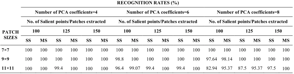
7. 2. 4. Varying the Number of PCA Coeficients

Table 4, gives the Recognition Rates for varying patch sizes and for various number of salient points/patches by varying the number of Principal Components as four, six and eight. It is evident from the Table 4 that for all the parameter variations patch size of 7×7 shows full recognition rates for all number of PCA coefficients. On increasing the patch size to 9×9 same performance is obtained for four and six number of PCA components but for eight number of PCA components, there are reduction in recognition rates when 100 patches are extracted. By increasing the patch size further, there is a drop in recognition rates for all four, six and eight number of PCA components. Of this three values, when the number of components is 4, there is a better recognition than for the more PCA component values such as six and eight. Hence, the lesser number of PCA components provides better results. On considering the number of Salient points, 100 salient points are enough to get better recognition for the cases of single scale and multi scale test images.

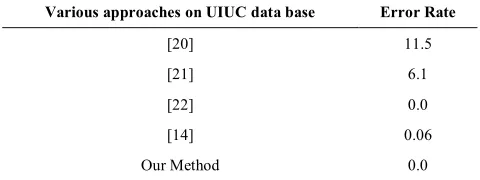
Table 5 shows the error rate performance for various techniques which uses UIUC datasets. In [19], Objects are modeled as flexible group of similar parts. In [20], Image patches are extracted around interest points and compared to the codebook. Matching patches then cast probabilistic votes, which lead to object hypotheses. In [21], regions of homogeneity are extracted using Similarity- Measure segmentation and the region descriptors used are the intensity values. Finally, Object categorization is done by Modified Adaboost algorithm. Our proposed technique gives error rate 0.0 when the patch size is 7×7.

TABLE 5. Error rates for various approaches on the UIUC car

datasets

Various approaches on UIUC data base Error Rate

[20] 11.5

[21] 6.1

[22] 0.0

[14] 0.06

Our Method 0.0

8. CONCLUSION

The proposed method focuses on Object Recognition in Complex Images under varying illumination and scaling conditions. This method uses Image Patches to extract the features. For the identification of patch locations, Wavelet based Salient points are used for better performance. In addition, this method outperforms the technique of using patches as the features directly and seems to be invariant to scaling and illumination conditions as they capture local structures well even in presence of uncertainties and noise conditions.

Though full recognition rate is obtained for various combinations, considering the computational complexity involved in number of salient points/patches, patch size, and number of PCA coefficients used, 100 salient points, 7×7 patch and four numbers of PCA coefficients are enough to obtain the full recognition rate in UIUC database. Thus, the proposed algorithm can be used for effectively recognizing objects under varying circumstances.

9. REFERENCES

1. Hegerath, A., Ney, I. H. and Seidl, T., "Patch-based object recognition", Diploma thesis, Human Language Technology and Pattern Recognition Group, RWTH Aachen University, Aachen, Germany, (2006)

2. Opelt, A., Pinz, A., Fussenegger, M. and Auer, P., "Generic object recognition with boosting", Pattern Analysis and Machine Intelligence, IEEE Transactions on, Vol. 28, No. 3, (2006), 416-431.

3. Shapiro, R. H. L. and Haralick, R., "Computer and robot vision",

Reading: Addison-Wesley, (1992).

4. Harris, C. and Stephens, M., "A combined corner and edge detector", in Alvey vision conference, Manchester, UK. Vol. 15, (1988), 50-58.

5. Loupias, E., Sebe, N., Bres, S. and Jolion, J.-M., "Wavelet-based salient points for image retrieval", in Image Processing, Proceedings. International Conference on, IEEE. Vol. 2, (2000), 518-521.

6. Seo, H. J. and Milanfar, P., "Using local regression kernels for statistical object detection", in Image Processing, ICIP, 15th IEEE International Conference on, IEEE, (2008), 2380-2383. 7. Seo, H. J. and Milanfar, P., "Training-free, generic object

detection using locally adaptive regression kernels", Pattern Analysis and Machine Intelligence, IEEE Transactions on, Vol. 32, No. 9, (2010), 1688-1704.

8. Takeda, H., Farsiu, S. and Milanfar, P., "Kernel regression for image processing and reconstruction", Image Processing, IEEE Transactions on, Vol. 16, No. 2, (2007), 349-366.

9. Seo, H. J. and Milanfar, P., "Face verification using the lark representation", Information Forensics and Security, IEEE Transactions on, Vol. 6, No. 4, (2011), 1275-1286.

10. Seo, H. J. and Milanfar, P., "Nonparametric bottom-up saliency detection by self-resemblance", in Computer Vision and Pattern Recognition Workshops, CVPR Workshops, IEEE Computer Society Conference on, IEEE, (2009), 45-52.

(8)

12. LeCun, Y., Huang, F. J. and Bottou, L., "Learning methods for generic object recognition with invariance to pose and lighting", in Computer Vision and Pattern Recognition, CVPR, Proceedings of the 2004 IEEE Computer Society Conference on, IEEE. Vol. 2, (2004), II-97-104.

13. Shaeiri, Z. and Ghaderi, R., "Modification of the fast global k-means using a fuzzy relation with application in microarray data analysis", International Journal of Engineering-Transactions C: Aspects, Vol. 25, No. 4, (2012), 283.

14. Mutch, J. and Lowe, D. G., "Object class recognition and localization using sparse features with limited receptive fields",

International Journal of Computer Vision, Vol. 80, No. 1, (2008), 45-57.

15. Deselaers, T., Hegerath, A., Keysers, D. and Ney, H., "Sparse patch-histograms for object classification in cluttered images", in Pattern recognition, Springer, (2006), 202-211.

16. Sebe, N. and Lew, M. S., "Comparing salient point detectors",

Pattern Recognition Letters, Vol. 24, No. 1, (2003), 89-96.

17. Duda, R. O., Hart, P. E. and Stork, D. G., "Pattern classification", John Wiley & Sons, (2012).

18. Ma, J., Zhao, Y. and Ahalt, S., "OSU SVM classifier matlab toolbox (ver 3.00)", Pulsed Neural Networks, (2002).

19. Fergus, R., Perona, P. and Zisserman, A., "Object class recognition by unsupervised scale-invariant learning", in Computer Vision and Pattern Recognition, Proceedings. IEEE Computer Society Conference on, IEEE. Vol. 2, No., (2003), 264 -271

20. Leibe, B., Leonardis, A. and Schiele, B., "Combined object categorization and segmentation with an implicit shape model", in Workshop on Statistical Learning in Computer Vision, ECCV. Vol. 2, No., (2004), 7-14.

21. Opelt, A. and Pinz, A., Object localization with boosting and weak supervision for generic object recognition, in Image analysis., Springer, (2005), 862-871.

Object Recognition based on Local Steering Kernel and SVM

R. AhilaPriyadharshini, S. Arivazhagan

Department of Electronics & Communication Engineering, Mepco Schlenk Engineering College, Sivakasi, Tamil Nadu, India

P A P E R I N F O

Paper history: Received 25 August 2012

Recivede in revised form 22 January 2013 Accepted 16 May 2013

Keywords: Object Recognition Salient Point Detector Patch Extraction Local Steering Kernel Principal Component Analysis

هﺪﯿﮑﭼ شور ﻪﺋارا هﺪﺷ ﺺﯿﺨﺸﺗياﺮﺑ ءﺎﯿﺷا ﺮﺑ سﺎﺳا هدﺎﻔﺘﺳا زا

Local Steering Kernels (LSK)

ﻪﺑ ناﻮﻨﻋ ﺗ ﻔﯿﺻﻮ ﺮﮕ ﻪﮑﺗ يﺎﻫ ﺮﯾﻮﺼﺗ ﺪﺷﺎﺑﯽﻣ . ﻪﺑ رﻮﻈﻨﻣ نﺎﺸﻧ نداد صاﻮﺧ ﻪﻄﻘﻧﮏﯾ زا ﺮﯾوﺎﺼﺗ ﻪﮐ رد نآ تاﺮﯿﯿﻐﺗ خر ﯽﻣ ﺪﻫد ، ﭻﭘ هدﺎﻔﺘﺳادرﻮﻣ

دﺮﯿﮔﯽﻣراﺮﻗ

. ياﺮﺑ اﺪﯿﭘ ندﺮﮐ ﻪﻄﻘﻧ ﺮﻈﻧدرﻮﻣ ، ﯽﻨﺘﺒﻣ ﺮﺑ زﺎﺳرﺎﮑﺷآ ﺟﻮﻣ ﯽ ﻪﻄﻘﻧ ﻪﺘﺴﺟﺮﺑ هدﺎﻔﺘﺳا ﯽﻣ دﻮﺷ . ،ﺲﭙﺳ شورزا (LSK) ﻪﺑ رﻮﻈﻨﻣ ﯽﺑﺎﯾﺖﺳد ﻪﺑ ﻞﺴﮑﯿﭘ

دﻮﺷﯽﻣهدﺎﻔﺘﺳابﻮﻠﻄﻣ

.

ﯽﮔﮋﯾو يﺎﻫ جاﺮﺨﺘﺳا هﺪﺷ

ﺪﺣزاﺶﯿﺑ

هدﻮﺑﻞﻣﺎﮐ ؛ ،ﻦﯾاﺮﺑﺎﻨﺑ ﻪﺑ رﻮﻈﻨﻣ ﺶﻫﺎﮐ ،دﺎﻌﺑا ﻪﯾﺰﺠﺗ و ﻞﯿﻠﺤﺗ ياﺰﺟا ﯽﻠﺻا ، شور ) PCA ( لﺎﻤﻋا ﯽﻣ دﻮﺷ . هوﻼﻋ ﺮﺑ ،ﻦﯾا ﺶﯾﺎﻤﻧ زﺮﻃ رﺎﺸﺘﻧا ﻞﺻاﻮﻓو عﺎﻔﺗراو لﻮﻠﺳ ﺎﻫ ﺶﯿﺑ زا PCA ﯽﺟوﺮﺧ ، زا ﻢﻫ هﺪﻨﮐاﺮﭘ ﺖﺳا . ﻪﻘﺒﻃ يﺪﻨﺑ درﻮﻣ هدﺎﻔﺘﺳا رد ﺎﺠﻨﯾا ﻦﯿﺷﺎﻣ رادﺮﺑ ) SVM ( ﻪﻘﺒﻃ يﺪﻨﺑ ﯽﻧﺎﺒﯿﺘﺸﭘ ﺖﺳا . ﺖﻣﻼﻋ ﻪﺼﺨﺸﻣ هﺎﮕﯾﺎﭘ هداد ﺎﺑ هدﺎﻔﺘﺳا زا ﮏﻧﺎﺑ ﯽﺗﺎﻋﻼﻃا وردﻮﺧ UIUC ﺖﺳا و ﺞﯾﺎﺘﻧ ﻪﺑ ﺖﺳد هﺪﻣآ ﺖﯾﺎﺿر ﺶﺨﺑ ﺖﺳا . ﺞﯾﺎﺘﻧ ﻪﺑ ﺖﺳد هﺪﻣآ ﺎﺑ هدﺎﻔﺘﺳا زا ﻪﺘﺴﻫ LSK ظﺎﺤﻟزا يﺎﻫﺮﺘﻣارﺎﭘ ﻒﻠﺘﺨﻣ ﺪﻨﻧﺎﻣ هزاﺪﻧا ،ﭻﭘ يداﺪﻌﺗ زا طﺎﻘﻧ ﻪﺘﺴﺟﺮﺑ ﺖﺒﺴﻧﻪﺑ ﺎﻫﭻﭘ ، ﺮﺘﻣارﺎﭘ حﻮﺿويﺎﻫ و ﺮﺘﻣارﺎﭘ هزاﺪﻧايﺎﻫ

ﺪﺷﺎﺑﯽﻣﻪﺴﯾﺎﻘﻣﻞﺑﺎﻗ

.