Numerical Approximation to Spherical Functions by Regularization method

ISSN :2394-2231 http://www.ijctjournal.org Page 57

Numerical Approximation to Spherical Functions by

Regularization method

Siyong Chen

1

, Congpei An

2

1,2_{(Department of Mathematics, Jinan University, Guangzhou, China. )}

---

************************

---Abstract:

In this paper, we apply Alternating Direction Method of Multipliers(ADMM) to solve a l1

-regularization optimization problem over the unit sphere. For different functions, we set up proper regularization operators. In particular, we consider approximation to Wendland function and cone function, with or without the presence of data errors. Based on choosing nodes as well conditioned spherical t-design, numerical experiments demonstrate approximation quality vividly.

Keywords —spherical polynomial approximation, ADMM, l₁-regularization.

---

************************

---I. INTRODUCTION

On the unit sphere, [1] introduces a spherical discrete least squares model with rotationally invariant regularization operators. This model includes a series of least squares model, such as

spherical polynomial interpolation,

hyperinterpolation and filtered hyperinterpolation. In this paper, we consider a class of spherical

1

-l regularization least squares approximation model

over the two-dimensional unit sphere

{

}

2 3 2 2 2

:= =( , , )T ∈ + + =1

x y z x y z

x

S :

(

)

2

1 1

( ) ( ) ( )

min λ ,

∈ _{= =}

− +

 

 



∑

∑



L

N N

j j L j

p

j j

p x f x R p x

P

(1)

where f is a given continuous function with values (possibly noisy) given at N points XN =

{

x₁,…,

}

_⊂ 2 N

x S . 2

:= ( )

L L S

P P is the linear space of spherical polynomial of degree ≤L. Regularazation operator R_L is a linear operator which can be chosen in different ways, and λ>0 is a parameter. Many different approximations are included in (1) through the freedom to vary the point sets X_N and the regularization operator R_L.

To simplify the model (1), we choose a basis for P_L. We take a basis of orthonormal spherical harmonics[2]

{

Yl,k l= …0, , ,L k= …1, ,2l+1 .

}

This orthogonal basis is normalized so that

0,1= ₄1_π

Y _{. Its dimension is}

0

dim( )=

∑

₌ (2 +1)

l l

L L

P

2

( 1)

= L+ .

The spherical harmonics Y_l,k with fixed l

forms a basis for the 2l+1-dimensional space H _l of homogeneous, harmonic polynomials of degree

l. The orthonormality is with respect to the L ₂ inner product

(

)

2 ₂

, :=

∫

( ) ( )

ω

( ),

f g _L f x g x d x

S

which induces the norm

(

)

2 2

1 2

:= ,

f _L f f _L . Then for

arbitrary p∈P_L , there is a unique vector

2

( 1) ,

(α ) +

= lk ∈ L

α such that

2 1

2 , ,

0 1

.

( ) α ( ),

+

= =

=

∑ ∑

∈

l

l l

l

k k L

k

p x Y x x S

Given a continuous function f , let f:=f(X_N)

be the column vector

[

( ),1 , ( )

]

.

= … T∈ N

N

f f

f x x

Let := ( )∈ (L+1)2×N

L L N

Y Y X be a matrix of

spherical harmonics evaluated at the points of X_N

with elements

, ( ), = …0, , , = …1, ,2 +1 ; = …1, , .

lk j l l

Y x L k j N

IJCT

ISSN :2394-2231 http://www.ijctjournal.org Page 58

For regularization operator, we consider the following two cases:

1) The first regularization operator R_L is defined in its most general rotationally invariant form by its action on

∈ _L

p P ,

2 2 2 1 , , 0 1 0 ( ) ( )( , )

2 1 _{( ) ( ) ( ),}

4 β β _π ω + = = = = + = ⋅

∑ ∑

∑ ∫

l

l l l

l

l l

l

l L

L k k

k L

p Y Y p

P p d

x x

x y y y

R _L

S

where x y⋅ denotes the euclidean inner product and P_l

denotes the orthogonal Legendre polynomials of degree l

which satisfies P_l

( )

1 =1 . In the last step we used the addition theorem for spherical harmonics[2]:

(

)

2 1 2 , , 1 2 1

( ) ( ) _4π , .

+

=

+

= ⋅ ∀ ∈

∑

l lk lk l l

k

Y xY y P x y x y S (2)

So, we have

(

)

T

( )= = T .

Lp x B YL L α RLα

R

where ( +1)2×( +1)2

∈ L L L

B is a positive semidefinite diagonal

matrix defined by

0 1 1 1

3 2 1

, , , , , , ,

: diag β β β β β β .

+

… …

 

=  

 14243 1424L 3L L

L B

The problem (1) can be reformulated as the following least squares problem:

2

( 1)

2

2 1

min

λ

,

λ

0.

+

∈

− + >

L

T T

L L

α

Y α f R α (3)

2) We consider a special case of (3): the regularization operator acts directly on the coefficients α, i.e. T = T .

L L

R α B α The problem (1) can be reformulated as the following least squares problem:

2

( 1)

2

2 1

min λ , λ 0.

+

∈

− + >

L

T T

L L

α

Y α f B α (4)

In the sequel, we introduce Alternating Direction Method of Multipliers to solve problem (3). The discussion of the choice of regularization operator is given in Section III. Section IV considers point set on sphere, testing functions, and numerical experiments on Wendland function and Cone function on the unit sphere.

II. ADMMMETHOD

Now, we illustrate Alternating Direction Method of Multipliers(ADMM)[3] to solve l₁ -regularization optimization problem (3). First, let

= T L

ζ R α. (3) can be transformed into the following constraint optimization problem

2 ( 1) 2 2 1 min s.t. . λ + ∈ + − − = L T L T L α ζ

Y α f

R α ζ 0

(5)

Then we form the augmented Lagrangian of (5)

(

)

1 2 2 2 2 ( , , ) ， ρ λ ρ = − + + − + −

T T T

L L

T L

L α ζy Y α f ζ y R α ζ

R α ζ

where ρ>0 is the penalty parameter. So, ADMM consists of the iterations

(

2 2

)

1

2 2

: argmin ,

2

ρ +

= − + − +

k T T k k

L L

α

α Y α f R α ζ u (6)

(

2

)

1 1

1 2

: argmin ,

2

ρ λ

+ ₌ +

+ − +

k T k k

L ζ

ζ ζ R α ζ u (7)

1 1 1

: .

+ + +

= + −

k k T k k

L

u u R α ζ (8)

where 1

ρ =

u y. In each iteration, we need to solve

two sub-problems (6)(7).

By the first order optimality conditions of (6), we obtain that its optimal solution α satisfies

(

2 T +ρ T

)

−

(

2 +ρ

(

k− k

)

)

= .

L L

L L L L α Y f R ζ u

Y Y R R 0

By solving the system of linear equations, we have

(

)

1

(

(

)

)

1 2 2 . ρ ρ − + = + + −

k T T k k

L L

L L L L

α Y Y R R Y f R ζ u (9)

For sub-problem (7), let k = T k+1+ k L

ν R α u . Since (7) is separable, we have

(

)

1 2

2

argmin λ ρ( ) ,

+ _{= + −}

i

k k

i i i i

ζ

ζ ζ ν ζ

where the first term

λ

ζ_i is not differentiable. By using the theory of subdifferential calculus[3], we can compute a closed-form solution, that is

( )

1 / : _{λ ρ} , + = k k

i S i

ζ ν

where S a_k( )=max

(

0,a−k

)

+min

(

0,a+k

)

. is the soft thresholding operator:

In summary, using ADMM algorithm for solving (5) is equivalent to solving a system of linear equations and using the soft thresholding operator alternately. Therefore, the iterations can be reformulated as follows:

(

)

1

(

(

)

)

1

1 /

1 1 1

2 2 : , : ( ), : . λ ρ ρ ρ − + + + + + + − + = = = + − k k T T L L

L L L L

k

k k

i i

k k T k k

L

S

Y f R ζ u

Y Y R R

α

ζ ν

u u R α ζ

IJCT

ISSN :2394-2231 http://www.ijctjournal.org Page 59

III. REGULARIZATIONOPERATOR

The regularization operator R is determined _L

by the choice of the diagonal matrix BL with

diagonal elements

β

_l. In the following, we present some interesting examples.

1) Filtered Regularization Operator: The diagonal element of the corresponding diagonal matrix B_L of this operator is defined as follows:

(

1

)

1, 0, , 1,

β_l = − = … −

l l

h L L (10)

where h x( ) is filter function. In this paper, we consider the following two _C∞ exponential filter function[4]:

• ₁

(

exp( 2 2( 1))

)

1

1, [0,1 / 2],

exp , (1/ 2,1),

( )

0, [1, ).

− −

−

∈



∈ =

∈ ∞



x x

x x h x

x

• ₂

(

2exp 1( ( 1))

)

1 2

1, [0,1 / 2],

1 exp , (1 / 2,1),

( )

0, [1, ).

− −

∈



− ∈

=

∈ ∞



x x

x x h x

x

In (10), we have excluded l=L because if l=L were allowed we would have β_L = ∞ and hence αL k_, =0.

2) Differential operator: The Laplace–Beltrami operator

*

∆ [2] is

(

)

* 2

2 2

1 1

: sin .

sinθ ∂θ θ ∂θ sin θ ∂φ

∆ = _{∂ ∂} +

∂

The spherical harmonics have an intrinsic characterization as the eigenfunctions of the Laplace-Beltrami operator *

∆ , that is,

*

, ( ) ( 1) , ( ).

∆ Y_lk x = −l l+ Y_lk x

It follows that _−∆* _{is a semipositive operator[2], and for}

any s>0 we may define (−∆*)s _by *

, ,

(−∆ )sY_lk( )x =[ (l l+1)]sY_lk( ).x

We used _(−∆*₎s _{as a regularization operator. The}

corresponding matrix B_L is then

3 2 1

0 ,2 ,2 ,2 , , [ ( 1)] , ,[ ( 1)]

diag .

+

… + … +

 

=  

 123 144424443

s s s s s s

L L

L L L L

B

This operator can recover the function with noise[5].

IV. NUMERICALEXPERIMENT

In this section we investigate spherical l₁ -regularization least squares approximation model to approximate some test functions over the sphere.

In this paper, we choose the spherical t-design with properly degree t as the point set X , which _N definition is as follows:

Definition 1[6]A point set X_N =

{

x₁,…,x_N

}

⊂S 2 is a spherical t-design, if it satisfies

2

1

1 _{( )} 1 _{( ) ( ) ,}

4

π

ω

=

= ∀ ∈

∑

N j

_∫

t

j

p p d p

N x S x x P (11)

where dω( )x denotes area measure on the unit sphere. That is, XN is a spherical t-design if a

properly scaled equal-weight quadrature rule with nodes at the points of X_N integrates all (spherical) polynomial up to degree t exactly.

In the following experiments, we assume X_N is well condition spherical t-design with t≥2L and

2

( 1)

= +

N t .

We use the following two test functions. The first one is Wendland function[7]:

(

)

6

1

1

( ) φ

=

=

∑

_{k i}− i

f x z x

where φ_k

( )

=φ%_k

( )

_δ k

r

r is normalized Wendland

function, (3 3) ( 12)

2 ( 1)

,

0

δ

_k = k+ Γ_Γk+k+

k

≥

and z1=( 1, 0, 0)T,

2=( 1,- 0, 0)T

z ,z3=( 0, 1, 0)T,z4=( 0, 1, 0)- T,

5=( 0, 0, 1)T

z ,z6=( 0, 0, - 1)T. In the following

experiments, we set k=2 and the corresponding original Wendland function is

( )

6 2

(1 ) (35 18 3) 3

φ

%k

r

= −r + r + r+ where

( )r ₊ =max{ , 0}r . The second function is the cone function f2[8]:

(

)

cone

arccos( )

2

2 1 , ( , )

0, otherwise,

⋅

 _{− ∈}

= =



c

c

r r

f f

x x _{x x}

C

where C(x_c, ) :r =

{

x∈S2 arccos( ,x x_c)≤r

}

is a spherical cap with center xc and radius

r

. This

function is continuous on 2

S but not differentiable on the boundary of the spherical cap C(xc, )r and

the center xc. In our numerical experiments, we set

(

1

)

2

1 1 2 2

, ,

= T

c

x and 1

2

=

r .

IJCT

• The uniform error of approximation is estimated by

2 2

( ) sup ( ) ( )

max ( ) ( ) ,

∈ ∈

− = −

≈ −

i N

L C L

x

i L i

x

f p f x p x

f x p x

X S

S

where X_N is a finite but large set of well distributed points over the sphere. In the following experiment, we choose X_N to be an equal area partitioning point set with N =50000 points[9]. • The L2-norm of approximation error is estimated

by

(

)

(

)

2 2

1/ 2 2

1/2 2

1

: ( ) ( ) ( )

4 _{( ) ( ) ,}

ω

π

=

− = −

≈ −

∫

∑

L L

m

j L j

j

f p f p d

f p

m

x x x

x x

L _S

The set

{

x₁,…,xm

}

is the nodes of the spherical

160-design with m=25921.

A. Filtered regularization operator for exact data

In this subsection, we report numerical results to compare different filter function. For a given L, we consider t=2L and set N =(t+1)2. We use both filter function h x₁( ) and h x₂( ) with β_l given by (10) and

λ

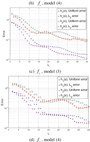
=1

Fig. 1 reports the uniform error and L2-error

of approximations for the functions f₁ and f₂ with 1, , 40

= …

L . Fig. 1 shows that model with filtered regularization operator with h x₁( ) has smaller uniform errors and L2-error than it with h x₂( ).

(a) f₁, model (3)

(b) f₁, model (4)

(c) f₂, model (3)

(d) f₂, model (4)

Fig. 1 Errors of model (3) and (4) with filtered regularization operator

B. Laplace–Beltrami regularization operator for contaminated data

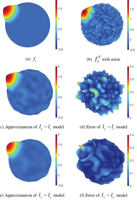
In this subsection, we report numerical results for reconstructing the nonsmooth function f₂ when the data has been contaminated with noise. We use model (4) with differential operator (s=2) and different values of

λ

.

Fig. 2(a) illustrates the function f2 while Fig.

2(b) shows the contaminated function

2 ( ) 2 ( )

δ _{= +δ}

f x f x , where for each x , δ( )x is a sample of a normal random variable with mean

0

µ= and standard deviation

σ

=0.2 . In this experiment, the choice of the regularization parameter

λ

is critical. We set the

λ

that achieve the minimal uniform error as the optimal

λ

.

The well condition spherical 50-design with

2601

=

N is used to recover the data with noise. As

a comparison, we choose the least squares model with l2-regularization term[1]:

(

)

2

(

)

1 1

2

( ) ( ) ( ) 0

min λ ,λ .

= =

∈ − + >

 

 



∑

j j

∑



L

N N

L j

j j

p

p x f x p x

P

R

IJCT

model is not as smooth as restoration by l2−l2

model. But, l2−l1 model recovers the non-smooth

edges of the spherical cap more accurately than

2− 2

l l model. At last, Fig. 3 reports the uniform and

2

-L errors for recovering the function f₂ from contaminated data.

(a) f2 (b) ₂

δ

f with noise

(c) Approximation of l2−l1 model (d) Error of l2−l1 model

(e) Approximation of l2−l2 model (f) Error of l2−l2 model

Fig. 2 Differential operator to recover 2

f from contaminated data.

Fig. 3 Errors of model (4) with differential operator

V.CONCLUSIONS

In this paper, we study the l1-regularization

optimization problem over the unit sphere. Based on variant regularization operators, we set up a class of spherical regularization least squares approximation model. We illustrate the algorithm, includes ADMM, to solve this approximation problem by using well conditioned spherical t-design as sampling point set. Finally, numerical experiments demonstrate the theoretical results can provide satisfactory approximation on the sphere, with or without errors on data. The results show that this model can approximate the smooth and non-smooth spherical functions well, especially at the non-smooth edge.

REFERENCES

[1] C. An, X. Chen, I. H. Sloan, and R. S. Womersley, “Regularized Least Squares Approximations on the Sphere Using Spherical Designs,” SIAM J. Numer. Anal., vol. 50, pp. 1513–1534, 2012. [2] C. Müller, Spherical Harmonics, vol. 17. Berlin, Heidelberg: Springer

Berlin Heidelberg, 1966.

[3] S. Boyd, N. Parikh, E. Chu, B. Peleato, and J. Eckstein, “Distributed Optimization and Statistical Learning via the Alternating Direction Method of Multipliers,” Found Trends Mach Learn, vol. 3, no. 1, pp. 1–122, Jan. 2011.

[4] F. Filbir and W. Themistoclakis, “Polynomial approximation on the sphere using scattered data,” Math. Nachrichten, vol. 281, no. 5, pp. 650–668, May 2008.

[5] W. Freeden, T. Gervens, and M. Schreiner, Constructive approximation on the sphere with applications to geomathematics. Oxford University Press on Demand, 1998.

[6] P. Delsarte, J.-M. Goethals, and J. J. Seidel, “Spherical codes and designs,” Geom. Dedicata, vol. 6, pp. 363–388, 1977.

[7] A. Chernih, I. H. Sloan, and R. S. Womersley, “Wendland functions with increasing smoothness converge to a Gaussian,” Adv. Comput. Math., vol. 40, no. 1, pp. 185–200, Feb. 2014.

[8] I. H. Sloan and R. S. Womersley, “Filtered hyperinterpolation: a constructive polynomial approximation on the sphere,” GEM - Int. J. Geomath., vol. 3, no. 1, pp. 95–117, Apr. 2012.