INTELIGENCIA ARTIFICIAL
http://journal.iberamia.org/
X and more Parallelism
Integrating LTL-Next into SAT-based Planning with
Trajectory Constraints While Allowing for Even
More Parallelism
Gregor Behnke and Susanne Biundo
Institute of Artificial Intelligence, Ulm University, D-89069 Ulm, Germany
{gregor.behnke, susanne.biundo}@uni-ulm.de
Abstract Linear temporal logic (LTL) provides expressive means to specify temporally extended goals as well as preferences. Recent research has focussed on compilation techniques, i.e., methods to alter the domain ensuring that every solution adheres to the temporally extended goals. This requires either new actions or an construction that is exponential in the size of the formula. A translation into boolean satisfiability (SAT) on the other hand requires neither. So far only one such encoding exists, which is based on the parallel∃-step encoding for classical planning. We show a connection between it and recently developed compilation techniques for LTL, which may be exploited in the future. The major drawback of the encoding is that it is limited to LTL without the X operator. We show how to integrate X and describe two new encodings, which allow for more parallelism than the original encoding. An empirical evaluation shows that the new encodings outperform the current state-of-the-art encoding.
Keywords: Temporally Extended Goals, Planning as SAT, Linear Temporal Logic.
1
Introduction
Linear temporal logic (LTL [18]) is a generic and expressive way to describe (state-)trajectory constraints. It is often used to specify temporal constraints and preferences in planning, e.g., to describe safety constraints, to state necessary intermediate goals, or to specify the ways in which a goal might be achieved. Most notably, the semantics of such constraints in PDDL 3.0 [11] is given in terms of LTL formulae, which is the de-facto standard for specifying planning problems.
Traditionally, LTL constraints are handled by first compiling them into an equivalent B¨uchi Automa-ton, and then translating the automaton into additional preconditions and effects for actions (see e.g. Edelkamp [8]). This compilation might be too expensive as the B¨uchi Automaton for a formulaφcan have up to 2|φ| states. Recent work proposed another compilation using Alternating Automata [20]. These
automata have only O(|φ|) states allowing for a guaranteed linear compilation. There are also planners that do not compile the model, but evaluate the formula during forward search, e.g., TALplanner [7], TLplan [1], or the work by Hsu et al. [12]. However, heuristics have to be specifically tailored to incor-porate the formula, or else the search becomes blind. TALplanner and TLplan even use the temporally extended goals for additional search guidance.
ISSN: 1137-3601 (print), 1988-3064 (on-line) c
Another option is to integrate LTL into planning via propositional logic. Planning problems can be translated into (a sequence of) boolean formulae. A temporally extended goal can then be enforced by adding additional clauses to this formula. So far only one such encoding has been developed by Mattm¨uller and Rintanen [17]. It uses an LTL to SAT translation from the model checking community, which assumes that only a single state transition is executed at a time. The main focus of their work lies on integrating the efficient∃-step encoding with this representation of LTL formulae. In the ∃-step encoding operators can be executed simultaneously, as long as they are all applicable in the current state, the resulting state is uniquely determined, and there is an ordering in which they are actually executable. Mattm¨uller and Rintanen presented alterations to the∃-step formula restricting the parallelism such that LTL formulas without the next-operator are handled correctly.
We point out an interesting relationship between the LTL encoding of Mattm¨uller and Rintanen and the Alternating Automaton encoding by Torres and Baier, showing that both use the same encoding technique, although derived by different means. This insight might prove useful in the future, e.g., to allow for optimisation of the propositional encoding using automata concepts. Next, we show how the propositional encoding by Mattm¨uller and Rintanen can be extended to also be able to handle the next-operatorX. We introduce a new concept – partial evaluation traces – to capture the semantics of the encoding with respect to an LTL formula and show that our extension is correct. Based on partial evaluation traces, we show that the restrictions posed by Mattm¨uller and Rintanen [17] on allowed parallelism can be relaxed while preserving correctness. We provide an alteration of their encoding allowing for more parallelism. We present an alternative encoding, also based on partial evaluation traces, which allows for even more parallelism by introducing intermediate timepoints at which the formula is evaluated. Our empirical evaluation of all encodings shows that our new encodings outperform the original one.
2
Preliminaries
2.1
Planning
We consider propositional planning without negative preconditions. This is known to be equivalent to STRIPS allowing for negative preconditions via compilation. Also note that all our techniques are also applicable in the presence of conditional effects. We do not consider them in this paper to keep the explanation of the techniques as simple as possible. For the extension to conditional effects, see Mattm¨uller and Rintanen [17].
LetA be a set of proposition symbols andLit(A) ={a,¬a|a∈A} be the set of all literals over A. An actionais a tuple a=hp, ei, wherep– the preconditions – is a subset ofA ande– the effects – is a subset ofLit(A). We further assume that the effects are not self-contradictory, i.e., that for no a∈A
botha and¬aare in e. A states is any subset ofA. An action a=hp, eiis executable ins, iffp⊆s. Executingainsresults in the state (s\ {a| ¬a∈e})∪ {a|a∈e}. A planning problemP =hA, O, sI, gi
consists of a set of proposition symbolsA, a set of operatorsO, the initial statesI, and the goalg⊆A.
A sequence of actionso1, . . . , on is a plan forP iff there exists a sequence of statess0, . . . , sn+1such that for everyi∈ {1, . . . , n+ 1}, oi is applicable insi, its application results in si+1,s0=sI, andg⊆sn+1. This sequence of states is called an execution trace.
2.2
Linear Temporal Logic
Formulae in Linear Temporal Logic (LTL) are constructed over a set of primitive propositions. In the case of planning these are the proposition symbolsA. LTL formulae are recursively defined as any of the following constructs, wherepis a proposition symbol andf andg are LTL formulae.
⊥ | > |p| ¬f |f∧g|f∨g|Xf|Xf˚ |Ef |Gf |f U g
X, ˚X,E,G, andU are called temporal operators. There are several further LTL-operators like ˚U,R, or
S andT [4]. Each of them can be translated into a formula containing only the temporal operatorsX, ˚
finite traces, which is commonly called LT Lf [6]. The encodings we present can easily be extended to
the infinite case (see Mattm¨uller and Rintanen [17]). The truth value of an LT Lf formulaφ is defined
over an execution traceσ= (s0, s1, . . . , sn) as [[φ]](σ) where
[[p]](s0, σ) =p∈s0 ifp∈A [[¬f]](σ) =¬[[f]](σ)
[[f∧g]](σ) = [[f]](σ)∧[[g]](σ) [[f∨g]](σ) = [[f]](σ)∨[[g]](σ) [[Xf]](s0, σ) = [[ ˚Xf]](s0, σ) = [[f]](σ)
[[Xf]](s0) =⊥ [[ ˚Xf]](s0) =>
[[Ef]](s0, σ) = [[f]](s0, σ)∨[[Ef]](σ) [[Gf]](s0, σ) = [[f]](s0, σ)∧[[Gf]](σ) [[Ef]](s0) = [[Gf]](s0) = [[f]](s0) [[f U g]](s0, σ) = [[g]](s0, σ)∨
([[f]](s0, σ)∧[[f U G]](σ)) [[f U g]](s0) = [[g]](s0)
The intuition of the semantics of temporal operators is: Ef – eventuallyf, i.e.,f will hold at some time, now or in the future, Gf – globallyf, i.e., f will hold from now on for ever,f U g –f untilg, i.e., gwill eventually hold and until that time f will always hold, andXf – nextf, i.e.,f holds in the next state of the trace. Since we consider the case of finite LTL, we have – in addition to standard LTL – a new operator: weak next ˚X. The formula Xf requires that there is a next state and that f holds in that state. In contrast, ˚Xf asserts that f holds if a next state exists; if there is none, ˚Xf is always true, taking care of the possible end of the state sequence.
As a preprocessing step, we always transform an LTL formulaφinto negation normal form without increasing its size, i.e., into a formula where all negations only occur directly before atomic propositions. This can be done using equivalences like¬Gf =E¬f. Next, we add for each proposition symbol a∈A
a new proposition symbol a. Its truth value will be maintained such that it is always the inverse of a. I.e. whenever an action has¬aas its effect, we add the effectaand when it has the effectawe add¬a. Lastly, we replace¬ain φwitha, resulting in a formula not containing negation.
Given a planning problemP and an LTL formula φ, LTL planning is the task of finding a plan π
whose execution traceσwill satisfyφ, i.e., for which [[φ]](σ). For a given LTL formulaφwe defineA(φ) as the set of predicates contained in φ andS(φ) to be the set of all its subformulae. We write [o]φ
e for
the intersections of the effects ofoand A(φ), i.e. all those effects that occur inφ.
3
State-of-the-art LTL
→
SAT encoding
As far as we are aware, there is only a single encoding of LTL planning problems into boolean satisfiability, developed by Mattm¨uller and Rintanen [17]. They adapted a propositional encoding for LTL developed by Latvala et al. [14] for bounded model checking. The main focus of Mattm¨uller and Rintanen’s work lies on integrating modern, non-sequential encodings of planning problems into the formula. The encoding models evaluating the LTL formula in timesteps, which correspond to the states in a trace. In Latvala et al.’s encoding (which was not developed for planning, but for a more general automata setting) only a single action may be executed at each timestep in order to evaluate the formula correctly. Research in translating planning problems into propositional formulae has however shown that such sequential encodings perform significantly worse than those that allow for a controlled amount of parallel action execution [19]. Mattm¨uller and Rintanen addressed the question of how to use the LTL encoding by Latvala et al. in a situation where multiple state transitions take care in parallel – as is the case in these planning encodings. They used the property of stutter-equivalence which holds for LT L−X (i.e. LTL
Their encoding, which we will denote with M&R’07, is based on the∃-step encoding of propositional planning by Rintanen et al. [19]. As such, we start by reviewing the∃-step encoding in detail. In this encoding the plan is divided into a sequence of timesteps 0, . . . , n. Each timesteptis assigned a resulting state using decision variablesatfor alla∈Aandt∈ {1, . . . , n+ 1}, each indicating that the proposition
symbol a holds at timestep t, i.e. after executing the actions at timestep t−1. The initial state is represented by the variablesa0. Actions can be executed between two neighbouring timestepstandt+ 1, which is represented by decision variables ot for allo ∈O and t∈ {0, . . . , n}. If ot is true the action o
is executed at timet. The encoding by Kautz and Selman [13] is then used to determine which actions are executable in atand how the state at+1 resulting from their application looks like. In a sequential encoding, one asserts for each timesteptthat at most oneotatom is true. Intuitively, this is necessary to ensure that the stateat+1 resulting from executing the actionsotis uniquely determined. Consider, e.g., a situation where two actionsmove-a-to-b and move-a-to-c are simultaneously applicable, but result in conflicting effects. Executing these two actions in parallel has no well-defined result. Interestingly, the mentioned constraint is not necessary in this case, as the encoding by Kautz and Selman already leads to an unsatisfiable formula. There are however situations, where the resulting state is well-defined, but it is not possible to execute the actions in any order. Consider two actionsbuy-aand buy-b, both requiring money, spending it, and achieving possession of aandb, respectively. Both actions are applicable in the same state and their parallel effects are well-defined, as they don’t conflict. It is not possible to find a sequential ordering of these two actions that is executable, as both need money, which won’t be present before executing the second action. This situation must be prohibited, which can easily be achieved by forbidding parallel action execution at all, as in the sequential encoding.
In the ∃-step encoding, executing actions in parallel is allowed. Ideally, we would like to allow any subsetSofotto be executable in parallel, as long as there exists a linearisation ofS that is executable in
the statestrepresented byatand all executable linearisations lead to the same statest+1. This property is however practically too difficult to encode [19]. Instead, the∃-step encoding uses a relaxed requirement. Namely, (1) all actions inS must be executable in st, then it chooses a total order of all actions O, (2)
asserts that if a set of actionsS is executable, it must be executable in that order, and (3) that the state reached after executing them in this order isst+1. The encoding by Kautz and Selman ensures the first and last property. The ∃-step encoding has to ensure the second property. It however does not permit all subsetsS⊆Oto be executable in parallel, but only those for which this property can be guaranteed. As a first step, we have to find an appropriate order of actions in which as many subsetsS ⊆O as possible can be executed. For this, the Disabling Graph (DG) is used. It determines which actions can be safely executed in which order without checking the truth of propositions inside the formula. In practice, one uses a relaxed version of the DG (i.e. one containing more edges), as it is easier to compute [19].
Definition 1. LetP =hA, O, sI, gibe a planning problem. An actiono1=hp1, e1iaffectsanother action
o2=hp2, e2iiff∃l∈A s.t. ¬l∈e1 andl∈p2.
A Disabling Graph DG(P)of a planning problem P is a directed graph hO, Eiwith E ⊆O×O that contains all edges(o1, o2)where o1 affectso2 and a state sexists that is reachable fromsI in which both
o1 ando2 are applicable.
The DG is tied to the domain itself and is not tied to any specific timestep, as such the restrictions it poses apply to every timestep equally. The DG encodes which actions disable the execution of other actions after them in the same timestep, i.e., we ideally want the actions to be ordered in the opposite way in the total ordering chosen by the∃-step encoding. If the DG is acyclic, we can execute all actions in the inverted order of the disabling graph, as none will disable an action occurring later in that order. If so, the propositional encoding does not need any further clauses, as any subsetS of actions can be executed at a timestep – provided that their effects do not interfere.
we know that there is a linearisation in which the chosen subsetS is actually executable. To ensure this property, Rintanen et al. introduced chains. A chainchain(≺;E;R;l) enforces that whenever an action
o inE is executed, all actions inR that occur afterain ≺cannot be executed. Intuitively,E are those actions that produce some effecta, while the actions inR rely on¬ato be true. The last argumentl is a label that prohibits interference between multiple chains.
chain(o1, . . . , on;E;R;l) =
^
{oi→dj,l|i < j, oi∈E, oj∈R,{oi+1, .., oj−1} ∩R=∅}
∪ {li→aj,l|i < j,{oi, oj} ⊆R,{oi+1, .., oj−1} ∩R=∅}
∪ {li→ ¬oi|oi∈R}
To ensure that for any SCCS ofDG(P) the mentioned condition holds for the chosen ordering ≺ofS, we generate for every proposition symbola∈A a chain with
Ea={o∈S|o=hp, eiand¬a∈e}
Ra={o∈S|o=hp, eianda∈p}
Based on the∃-step encoding, Mattm¨uller and Rintanen [17] added support for LTL formulaeφ by exploiting the stutter-equivalence ofLT L−X. This stutter-equivalence ensures that if multiple actions are
executed in a row but don nott change the truth of any of the predicates inA(φ), the truth of the formula is not affected, i.e., the truth of the formula does not depend on how many of these actions are executed in a row. Consequently the formula only needs to be checked whenever the truth of propositions inA(φ) changes. Their construction consists of two parts. First, they add clauses to the formula expressing that the LTL formula φis actually satisfied by the trace restricted to the states where propositions in A(φ) change. These states are the ones represented in the ∃-step encoding by at atoms. Second, they add
constraints to the ∃-step parallelism s.t. in every timestep the first action executed according to≺that changes proposition symbols in A(φ) is the only one to do so. Other actions in that timestep may not alter the state with respect toA(φ) achieved by that first action, but can assert the same effect.
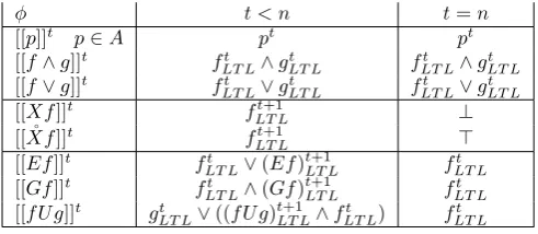
In their paper, they provide a direct translation ofφinto a proposition formula. In practice however, this formula cannot be given to a SAT solver, as it requires a formula in conjunctive normal form (CNF). The formula given in the paper is not in CNF and translating it into CNF can lead to a CNF of exponential size. They instead introduce additional variables [16], allowing them to generate (almost) a CNF1. For every sub-formulaψ∈ S(φ) and every timesteptthey introduce the variableψt
LT L, stating thatψholds
for the trace starting at timestept. They then assert: (1) thatφ0
LT L holds and (2) that for everyψtLT L
the consequences must hold that makeψtrue for the trace starting at timet. The latter is expressed by clausesψt
LT L→[[ψ]]t, where [[ψ]]tis given in Tab. 1. Note that the M&R’07 encoding cannot handle the
next operators X and ˚X, as they are sensitive to stuttering, i.e., stutter-equivalence does not hold for formulae that containX or ˚X. We have added the encoding forX [14]. In addition, we have restricted the original encoding from infinite to finite LTL-traces and added a new encoding for ˚X. Note that the M&R’07 encoding will lead to wrong results if used with the presented encoding of the X and ˚X
operators. It is however correct, if used in conjunction with a sequential encoding [14]. We show in Sec. 5 how the M&R’07 encoding can be changed to handleX and ˚X correctly. Lastly, clauses need to be added in order to ensure that actions executed in parallel do not alter the truth of propositions inA(φ) – except for the first action that actually changes them. The extension of the ∃-step encoding achieving this is conceptually simple, as it consists of only two changes to the original encoding:
1. Add for every two actionso1, o2which are simultaneously applicable the edge (o1, o2) to the DG iff [o2]φe\[o1]φe 6=∅, i.e., o2 would change more thano1 with respect toA(φ).
2. Add for every literall∈Lit(A(φ)) and SCC ofDG(P) with its total order≺the chainchain(≺;Elφ;Rφl;φl)
with
φ t < n t=n
[[p]]t p∈A pt pt
[[f∧g]]t ft
LT L∧gLT Lt fLT Lt ∧gtLT L
[[f∨g]]t ft
LT L∨gLT Lt fLT Lt ∨gtLT L
[[Xf]]t ft+1
LT L ⊥
[[ ˚Xf]]t ft+1
LT L >
[[Ef]]t ft
LT L∨(Ef)tLT L+1 fLT Lt
[[Gf]]t ft
LT L∧(Gf)tLT L+1 fLT Lt
[[f U g]]t gt
LT L∨((f U g) t+1
LT L∧fLT Lt ) fLT Lt
Table 1: Transition rules for LTL formulae
(a) Elφ={o∈O|o=hp, eiandl6∈e}
(b) Rφl ={o∈O|o=hp, eiandl∈e};
Mattm¨uller and Rintanen [17] have proven that these clauses suffice to ensure a correct and complete encoding.
4
Alternating Automata and M&R’07
In recent years, research on LTL planning focussed on translation based approaches. There, the original planning problem is altered in such a way that all solutions for the new problem adhere to the formula (e.g. Baier and McIlraith [2] and Torres and Baier [20], see Camacho et al. [5] for an overview). Traditionally, these approaches translate the LTL formula into a B¨uchi automaton (essentially a finite state machine, with a specific accepting criterion for infinite traces) and then integrate the automaton into the model. The major drawback of these translations is that the B¨uchi automaton for an LTL formula can have up to 2|φ|many states.
Torres and Baier [20] proposed a translation diverging from the classical LTL to B¨uchi translation. They instead based it on Alternating Automata, which are commonly used as an intermediate step when constructing the B¨uchi automaton for an LTLφformula (see e.g. Gastin and Oddoux [10]). Alternating Automata have a guaranteed linear size in|φ|, but have a more complex transition function.
Definition 2. Given a set of primitive propositions A, an alternating automaton is a 4-tuple A = (Q, δ, I, F)where
• Qis a finite set of states
• δ : Q×2A → B+(Q) is a transition function, where B+(Q) is the set of positive propositional formulas over the set of statesQ, i.e., those formulae containing only∨and∧.
• I⊆Qis the initial state
• F ⊆Qis the set of final states.
A run of an alternating automaton over a sequence of sets of propositions (execution trace)(s1, . . . , sn)
is a sequence of sets of states(Q0, . . . , Qn) such that
• Q0=I
• ∀i∈ {1, . . . , n}:Qi|=Vq∈Qi−1δ(q, si)
The alternating automaton accepts the trace iffQn ⊆F
Torres and Baier [20] generate an alternating automaton for an LTL formula φ as follows. They chooseQas the set of sub-expressions ofφstarting with a temporal operator plus a stateqF representing
time on we have to fulfill the formula q. The automaton is given as Aφ = (Q, δ,{qφ},{qF}) where
Q={qα|α∈ S(φ)} ∪ {qF}and the transition functionδis defined as follows:
δ(ql, s) =
(
> ifl∈s
⊥ ifl6∈s δ(qF, s) =⊥
δ(qf∨g, s) =δ(qf, s)∨δ(qg, s)
δ(qf∧g, s) =δ(qf, s)∧δ(qg, s)
δ(qXf, s) =qf
δ(qXf˚ , s) =qF ∨qf
δ(qEf, s) =δ(f, s)∨qEf
δ(qGf, s) =δ(f, s)∧(qGf ∨qF)
δ(qf U g, s) =δ(qg, s)∨(δ(qf, s)∧qf U g)
Note that we have to enumerate all states that are relevant to the formula, i.e., all states s ⊆ 2A(φ), to construct the formula. Using the Alternating Automaton as the basis for a translation leads to a guaranteed linear increase in size when constructing the translated planning problem. This is due to the fact that the encoding does not actually has to construct the automaton, but only has to simulate its states. We will elaborate on this later. Also, it was demonstrated that the new encoding is more efficient than other current translation techniques [20].
A drawback of their translation was the need for introducing additional actions, performing bookkeep-ing on the current state of the alternatbookkeep-ing automaton. A translation into SAT, on the other hand, will not have this drawback, as we will show. We will again extend the∃-step encoding and call the encoding AA (Alternating Automaton). The restriction posed on parallelism by M&R’07 does not depend on the encoding of the formula itself as long as it does not contain the X or ˚X operators2. We introduce new decision variables qt for each state q ∈ Q and timestep t, signifying that the automaton Aφ is in
state q after executing the actions of timestep t. To express the transition function of the Alternating Automaton, we use formulae of the form qt∧V
a∈sa
→δ(q, s) for each stateq of the automaton and set of propositionss. We also replace each occurrence of a state qf in δ(q, s) with the decision variable
qtf+1 and introduce intermediate decision variables to break down complex formulae as in the M&R’07 encoding. The following theorem holds by construction.
Theorem 1. AA in conjunction with M&R’07’s∃-step encoding is correct for LT L−X.
We here want to point out that the AA encoding is not (as the one by Torres and Baier [20]) polynomial in the size of the formula. The reason lies in the explicit construction of the alternating automaton, which requires a single transition for every possible state that might be relevant to the formula, i.e., for every subset of A(φ). The translation encoding by Torres and Baier circumvents this construction by adding new operators, which can evaluate the necessary expression during planning. I.e. they have actions for each transition rule δ(·,·), which produce the right-hand sides of these above equations as their effects. Lastly, they introduce synchronisation actions to ensure that δ(·,·) is fully computed before another “real” action is executed.
If we apply this idea to the AA encoding, we would end up with the M&R’07 encoding. Since the states of the automaton are the sub-formulae ofφstarting with a temporal operator, these decision variables are identical to the ψt
LT L variables of the M&R’07 encoding, whereψstarts with a temporal operator. The
encoding by Torres and Baier also needs to introduce state variables for every sub formulae not starting with a temporal operator to represent the step-wise computation of δ(·,·) correctly. If translated into propositional variables, these correspond to theψt
LT L variables of M&R’07, whereψdoes not start with
a temporal operator. Lastly, the transition rules for both encodings are identical.
As such, the M&R’07 encoding can also be interpreted as a direct translation of an Alternating Au-tomaton into propositional logic using the compression technique of Torres and Baier [20]. Interestingly,
2The actual encoding of the formula can be exchanged in the proof of their main theorem as long as a similar version of
the original proof showing correctness of the LTL-part of the M&R’07 encoding by Latvala et al. [14] does not rely on this relationship to Alternating Automata, neither do they mention this connection. We think it is an interesting theoretical insight, as it might enable to further improve LTL encodings, e.g., based on optimisations of the Alternating Automaton.
5
X, Parallelism, and Partial Evaluation
We have noted that both M&R’07 and AA cannot handle LTL formulae containing theXor ˚X operators in conjunction with the∃-step encoding. They are however correct if used together with the sequential encoding, where only a single action can be executed at each timestep. In order to derive extensions that can handleX and ˚X, we first present a new theoretical foundation for both encodings. We will use the fact that in M&R’07, we know which parts of the formula are made true at which time and by which propositions. To formalise this, we introduce evaluation traces, which specify how an LTL formula is fulfilled over a trace.
Definition 3. Let φ be an LTL formula. We call a sequence ψ = (f0, . . . , fn) with fi ⊆ S(φ) an
evaluation trace forφiffφ∈f0 and for alli∈ {0, . . . , n}holds 1. if f∨g∈fi thenf ∈fi org∈fi
2. if f∧g∈fi thenf ∈fi andg∈fi
3. if Xf∈fi theni < n andf ∈fi+1 4. if Xf˚ ∈fi theni=n orf ∈fi+1
5. if Ef ∈fi thenf ∈fi or i < nandEf ∈fi+1 6. if Gf∈fi thenf ∈fi and if i < nthenGf ∈fi+1
7. if f U g∈fi theng∈fi ori < nandf ∈fi andf U g∈fi+1
A trace π= (s0, . . . , sn) satisfies an evaluation trace ψ = (f0, . . . , fn) iff for all a∈fi∩A also a ∈si
holds.
The following theorem follows directly, as the definition just emulates checking an LTL formula.
Theorem 2. An execution traceπsatisfies an LTL formulaφiff an evaluation traceψforφexists that satisfiesπ.
In M&R’07, the LTL formula is only evaluated after a set of parallel actions have been executed. To capture this, we define partial evaluation traces.
Definition 4. Letπ= (s0, . . . , sn)be an execution trace andφand LTL formula. We call an evaluation
traceθ= (f0, . . . , fl)with l≤na partial evaluation trace (PET) for πif a sequence of indices0 =i0<
i1< ... < il=n+ 1 exists such that for eachk∈ {0, . . . , l−1}holds
sik∩(fk∩A) =· · ·=sik+1−1∩(fk∩A)
and ifXf ∈fk or Xf˚ ∈fk andk >0 thenik−1+ 1 =ik. The PET θ is satisfied by the execution trace
π, iff the execution trace(si1−1∩f0∩A, . . . , sil−1∩fl∩A)satisfies θin the sense of Def. 3.
Theorem 3. Let πbe a trace andθ be an PET for the formulaφon π. Ifπsatisfiesθ, thenπ satisfies
φ.
Proof. We need to show that the PET ψ = (f0, . . . , fl) can be extended to a full evaluation trace on
π= (s0, . . . , sn), s.t. π satisfies that evaluation trace. If so, we can apply Thm. 2 and conclude that π
also satisfiesφ. Leti0, . . . , il be the indices of Def. 4 for whichθis a PET. We claim that
θ∗= (
i1−i0times z }| {
f0, . . . f0,
i2−i1times z }| {
f1, . . . , f1, . . . ,
il−il−1times z }| {
fl, . . . , fl )
is an evaluation trace that satisfiesπ, and thatπsatisfiesφ. First we show thatθ∗is an evaluation trace. We start by proving the enumerated properties of Def. 3. Consider the ith elementf∗ ofθ∗ and letf∗∗
be thei+ 1th element (if such exists). 1. trivially satisfied
2. trivially satisfied
3. Xf ∈ f∗. We know that f∗ is the only repetition some fj in the trace, as θ is a PET. Also
f∗∗=fj+1. Consequently f ∈f∗∗. In casef∗∗ does not exist,θcannot be an PET.
4. ˚Xf ∈f∗. We know thatf∗ is the only repetition of some fj in the trace, asθ is a PET. In case
f∗∗ does not exist, we have nothing to show. Else,f∗∗=fj+1 andf ∈f∗∗.
For the last three requirements relating to the temporal operatorsE,G, andU, we can distinguish three cases depending on where f∗ is situated in the sequenceθ∗
• f∗is the last element of θ∗:
5. ifEf ∈f∗ thenf ∈f∗, as θis a PET.
6. ifGf ∈f∗ thenf ∈f∗, asθ is a PET. 7. iff U g∈f∗ theng∈f∗, as θis a PET.
• f∗ 6= f∗∗, i.e., the last repetition of f∗. We know that f∗ = fj and f∗∗ = fj+1 for some j ∈
{0, . . . , l−1}.
5. ifEf ∈f∗ then eitherf ∈fj=f∗ orEf ∈fj+1=f∗∗ 6. ifGf ∈f∗ thenf ∈fj =f∗and Gf∈fj+1=f∗∗
7. iff U G∈f∗ then eitherg∈fj+1=f∗∗ orf ∈fj =f∗and f U g∈fj+1=f∗∗
• iff∗=f∗∗
5. ifEf ∈f∗ thenEf ∈f∗∗
6. ifGf ∈f∗ thenGf ∈f∗∗ andf ∈f∗
7. iff U g∈f∗ then eitherg∈f∗, orf ∈f∗, but then alsof U G∈f∗∗, sincef∗=f∗∗ φ∈f0holds as θis a PET, which concludes conclude the proof that θ∗ is an evaluation trace.
Lastly, we have to show thatθ∗satisfies π, i.e., we have to show, for each timestepj∈ {0, . . . n}and
everya∈Awhich is true in theith element ofθ∗, thata∈sj holds. Consider first the indices of the last
repetitions of eachfk, i.e., the statessik−1. Sinceθis a PET, it satisfies (si1−1∩f0∩A, . . . , sil−1∩fl∩A),
so it satisfies the required property for all time-steps ik−1. Consider any other timestept and its next
timestep in the PETik−1 (which always exists, since the last index is equal ton). Since θ is a PET,
we know that st∩(fk−1∩A) = sik−1∩(fk∩A). We have chosen to set the tth element of θ ∗ to f
k.
Since sik−1∩(fk∩A) satisfies the required property forfk, so mustst∩(fk∩A) and thusst itself (it
can have only more true predicates).
• exactOnet– exactly one action is executed at time t
• atLeastOnet – at least one action is executed at timet
• atM ostOnet– at most one action is executed at timet
• nonet– no action is executed at any time ≥t
To enforce the semantics of these variables, we add the following clauses per timestep:
∀o∈O:nonet→ ¬ot nonet→nonet+1 atLeastOnet→ _
o∈O
ot
exactOnet→atLeastOnet∧atM ostOnet
Encoding theatM ostOnetatom is a bit more complicated. A native encoding requiresO(|O|2) clauses. There are however better encodings for the at most one constraint in SAT. We have chosen the log-counter encoding, which introduces log(|S|) new variables while only requiring|S|log(|S|) clauses [9]. To ensure the semantics of the atom atM ostOnet, we add it as a guard to the log-counter encoding, i.e., we add
¬atM ostOnet to every clause. IfatM ostOnetis required to be true, the log-counter clauses have to be satisfied, i.e., at most one action atom can be true. IfatM ostOnetcan be false, we can simply set it to⊥
thereby satisfying all log-counter clauses. We lastly setexactOnet fort=−1 to>andatLeastOnen+1 to false. Based on these new variables, we can add the constraints necessary for evaluating X and ˚X
correctly under the∃-step encoding. For each timestept, we add
(Xf)tLT L→exactOnet−1∧ft+1∧atLeastOnet
( ˚Xf)tLT L→exactOnet−1
( ˚Xf)tLT L→(ft+1∧atLeastOnet)∨nonet
A valuation of this encoding represents a partial evaluation trace satisfied by the execution trace of its actions. By applying Thm. 3, we know that a satisfying evaluation trace for the plan exists. Showing completeness for the encoding is trivial, since a sequential assignment satisfies the formula for every plan. We will also call this extended encoding M&R’07 in our evaluation, as it is exactly identical to this one, provided noX or ˚X operator is present.
So far, we have not used the – in our view – most significant improvement: Relaxing the restrictions on parallelism to only those actually needed by the current formula. Doing so based on our theorem is surprisingly easy. Consider a timestep of the M&R’07 encoding, in which actions can be executed in parallel, which are given an implicit order≺by the∃-step encoding. For each literall∈Lit(A(φ)) a chain ensures that the action changing it is applied first, i.e., that the “first” action of a timestep performs all changes relevant to the whole formula and can thus check the formula only in the resulting state. By applying Def. 4 and Thm. 3, we have to ensure this property only for those proposition symbols that need to be evaluated after the actions have been executed, i.e., for all atLT L+1 that are true. We can do this simply by adding the literal¬at
LT Las a guard (simiar toatM ostOne
t) to every clause in the chains
chain(≺;Elφ;Rlφ;φa) and chain(≺;E φ l;R
φ
l;φ¬a). If we have to make the literal atLT L true, the chains
become active, if not they are inactive (as they are trivially satisfied by ¬at
LT L). We will denote this
improved encoding with Improved-M&R’07.
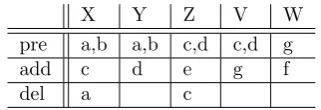
To illustrate the effects of the improved M&R’07 encoding, consider the following planning problem. There are six proposition symbolsa, b, c, d, eand f, of whicha andb are true in the initial state and
X Y Z V W pre a,b a,b c,d c,d g
add c d e g f
del a c
Table 2: Actions in the example domain
X
Y Z
V W
Figure 1: Extended disabling graph for the example domain.
the encoding correctly detects that there is a state in which aand dare true simultaneously3 after the action Y has been executed and that thusEf has to hold after executing Y. In the plan for the improved encoding, the solver can simply choose to achieveEf after{Y,X}has been executed. This way the solver is never forced to achieve¬aor¬dand can thus completely ignore the associated constraints, i.e., chains.
6
Parallelism with Tracking
There is however still room for more parallelism even compared to the improved M&R’07 encoding. The key observation is that in many domains only a few actions actually influence the truth of variables in an LTL formula, and that those that do are usually close to each other in a topological ordering of the inverse disabling graph. The∃-step semantic guarantees that if actions are executed in parallel, they can be sequentially executed in this order. Let this ordering be (o1, . . . , on). We can divide it into blocks,
such that for each block (oi, . . . , oj) it holds that
[oi]φe ⊇[oi+1]φe ⊇ · · · ⊇[oj]φe
Along the actions in a block the effects that contain predicates in A(φ) can only “decrease”. A block forms a set of actions that can always – without further checking at runtime – be executed in parallel in the M&R’07 encoding. The number of such blocks is surprisingly small for most domains (see Tab. 3). We denote withB= ((o1, . . . , oi), . . . ,(oj, . . . , on)) the sequence of blocks for a given ordering of actions.
If an action from a block has been executed, at least (usually more) the first action of the next block cannot be executed anymore in the same timestep, as it would change the truth of some a ∈ A(φ), even though it would be possible in the pure∃-step encoding. We present a method to circumvent this restriction on parallelism. Instead of restricting the amount of parallel actions executing inside a timestep, we (partially) trace the truth of an LTL formula within that timestep to allow maximal parallelism. This is based on the insight that all proofs by Mattm¨uller and Rintanen [17] do not actually require an action to be present at any timestep, i.e., the set of actions executed in parallel can also be empty. So, conceptually, we split each timestep into|B|many timesteps and restrict the actions in theith splitted step to be those of the ith block. Then we use the M&R’07 encoding, without the need to add chain-clauses apart from those of the∃-step encoding, as they are automatically fulfilled. The resulting encoding would be sound and complete for LTL formulae without X and ˚X by virtue of the results proven by Mattm¨uller and Rintanen [17].
We can however improve the formula even further. In the proposed encoding, we would compute the state after each block using the Kautz&Selman encoding. This is unnecessary, as we know from the
∃-step encoding, that we only need to compute the state again after all blocks of one original timestep have been executed. We only need to trace the truth of propositions in A(φ) between blocks. For that we don not need to check preconditions – they are already ensured by the∃-step encoding. We end up with the∃-step encoding, where we add at every timestep a set of intermediate timepoints at which the
truth of propositions inA(φ) and the truth of the LTL formulaφis checked. Thus we call this encoding OnParallel.
As we have noted above, this construction works only for the original M&R’07 encoding, as supporting theX and ˚X requires to be able to specify that in the next timestep some action must be executed. This might not be possible with splitted timesteps, as the next action to be executed may only be contained in a timestep|B|steps ahead. Luckily, we can fix this problem by slightly altering the encoding we used to track the truth ofX and ˚X operators.
(Xf)t→atM ostOnet−1∧((atLeastOneit∧fLT Lt+1)∨
(nextN onet+1∧(Xf)tLT L+1 ))
( ˚Xf)t→atM ostOnet−1∧((fLT Lt+1 ∧atLeastOnet)∨
(nextN onet+1∧( ˚Xf)tLT L+1 )∨nonet))
The semantics ofnoneAttis ensured by clausesnextN onet→ ¬otfor alli∈O. Lastly, we add¬XfLT Ln++11
for any Xf ∈ S stating that a next-formula cannot be made true at the last timestep. This would otherwise be possible, sinceatM ostOnen could simply be made true. The OnParallel encoding is correct by applying Thm. 3.
7
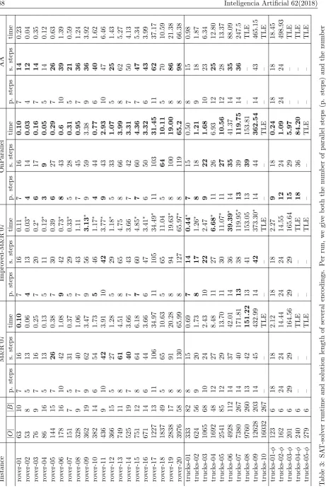
Evaluation
We have conducted an evaluation in order to assess the performance of our proposed encodings. We used the same experimental setting as Mattm¨uller and Rintanen [17] in their original paper. We used the domainstrucksandroverfrom the preference track of IPC5 (the original paper considered onlyrover), which contain temporally extended goals to specify preference. In these domains, temporally-extended goals are formulated using the syntax of PDDL 3.0 [11]. We parse the preferences and transform them into LTL formulae using the patterns defined by Gerevini and Long [11]. As did Mattm¨uller and Rintanen, we interpret these preferences as hard constraints and randomly choose a subset of three constraints per instance4. To examine the performance of our encoding forXand ˚X, we have also tested the instances of thetrucksdomain with a formula that contains these operators. We have used the following formula5:
φ=∀?l−Location?t−T ruck:G(at(?l,?t)→X˚(¬at(?l,?t)∨X˚¬at(?l,?t)))
It forces each truck to stay at a location for at most one timestep – either it leaves the location right after entering it, or in the next timestep. The domain contains an explicit symbolic representation of time, which is used in temporal goals. When planning withφ, the number of timesteps is never sufficed to find a plan satisfyingφ. We have therefore removed all preconditions, effects, and action parameters pertaining to the explicit representation of time. As a result, the domain itself is easier than the original one. We denote these instances in the evaluation with trucks-XY-φ.
Each planner was given 10 minutes of runtime and 4GB of RAM per instance on an Intel Xeon E5-2660 v3. We’ve used the SAT solver Riss6 [15], one of the best-performing solvers in the SAT Competition 2016. We have omitted results for all the trucks instances 11−20, as no planner was able to solve them. Table 3 shows the results of our evaluation. We show per instance the number of ground actions and blocks. The number of blocks is almost always significantly smaller than the number of ground operators. In the largestrover instance, only≈1.4% of operators start a new block. For thetrucksdomain this is≈1.7% for the largest instance.
For every encoding, we show both the number of parallel steps (i.e. timesteps) necessary to find a solution, as well as the time needed to solve the respective formula and the number of sequential plan steps found by the planner. In almost all instances the OnParallel encoding performs best, while there are some where the improved M&R’07 encoding is faster. Our improvement to the M&R’07 encoding almost always leads to a faster runtime. Also, the improved parallelism actually leads to shorter parallel plans.
4Mattm¨uller and Rintanen [17] noted that it is impossible to satisfy all constraints at the same time and that a random
sample of more than three often leads to unsolvable problems. If a sample of 3 proved unsolvable we have drawn a new one.
In approximately half of the instances we can find plans with fewer parallel steps. In the experiments with the formulaφ containing the ˚X operator, this is most pronounced. The OnParallel encoding cuts the number of timesteps by half and is hence significantly faster, e.g., on trucks-03-φwhere the runtime is reduced from 165s to 6s. On the other hand, the sequential plans found are usually a few actions longer, although the same short plan could be found – this result is due to the non-determinism of the SAT solver.
8
Conclusion
In this paper, we have improved the state-of-the-art in translating LTL planning problems into proposi-tional formulae in several ways. We have first pointed out an interesting theoretical connection between the propositional encoding by Mattm¨uller and Rintanen [17] and the compilation technique by Torres and Baier [20]. Next, we have presented a new theoretical foundation for the M&R’07 encoding – partial evaluation traces. Using them, we presented (1) a method to allow theX and ˚Xoperators in the M&R’07 encoding, (2) a method to further improve the parallelism in the M&R’07 encoding, and (3) a new encod-ing for LTL plannencod-ing. In an evaluation, we have shown that both our improved M&R’07 encodencod-ing and the OnParallel encoding perform empirically better than the original encoding by Mattm¨uller and Rintanen. We plan to use the developed encoding in a planning-based assistant [3] for enabling the user to influence the instructions he or she is presented by the assistant, which in turn are based on the solution generated by a planner. Instructions given by the user can be interpreted as LTL goal and integrated into the plan using the presented techniques.
Acknowledgement
References
[1] Fahiem Bacchus and Froduald Kabanza. Using temporal logics to express search control knowledge for planning. Artificial Intelligence, 116(1-2):123–191, 2000.
[2] Jorge Baier and Sheila McIlraith. Planning with first-order temporally extended goals using heuristic search. InProceedings of the 21st National Conference on AI (AAAI 2006), pages 788–795. AAAI Press, 2006.
[3] Gregor Behnke, Marvin Schiller, Matthias Kraus, Pascal Bercher, Mario Schmautz, Michael Dorna, Wolfgang Minker, Birte Glimm, and Susanne Biundo. Instructing novice users on how to use tools in DIY projects. InProceedings of the 27th International Joint Conference on Artificial Intelligence and the 23rd European Conference on Artificial Intelligence (IJCAI-ECAI 2018), pages 5805–5807. IJCAI, 2018.
[4] Armin Biere, Keijo Heljanko, Tommi Junttila, Timo Latvala, and Viktor Schuppan. Linear encodings of bounded LTL model checking. Logical Methods in Computer Science, 2(5):1–64, 2006.
[5] Alberto Camacho, Eleni Triantafillou, Christian Muise, Jorge A. Baier, and Sheila A. McIlraith. Non-deterministic planning with temporally extended goals: Ltl over finite and infinite traces. In Proceedings of the 31st National Conference on AI (AAAI 2017), pages 3716–3724. AAAI Press, 2017.
[6] Giuseppe De Giacomo and Moshe Y. Vardi. Linear temporal logic and linear dynamic logic on finite traces. InProceedings of the 23rd International Joint Conference on Artificial Intelligence (IJCAI 2013), pages 854–860. AAAI Press, 2013.
[7] Patrick Doherty and Jonas Kvarnstr¨om. TALPLANNER – A temporal logic-based planner. The AI Magazine, 22(3):95–102, 2001.
[8] Stefan Edelkamp. On the compilation of plan constraints and preferences. InProceedings of the 16th International Conference on Automated Planning and Scheduling (ICAPS 2006), pages 374–377. AAAI Press, 2003.
[9] Alan Frisch, Timothy Peugniez, Anthony Doggett, and Peter Nightingale. Solving non-boolean satisfiability problems with stochastic local search: A comparison of encodings.Journal of Automated Reasoning (JAR), 35(1-3):143–179, 2005.
[10] Paul Gastin and Denis Oddoux. Fast ltl to b¨uchi automata translation. In Proceedings of the 13th International Conference on Computer Aided Verification (CAV 2001), pages 53–65. Springer-Verlag, 2001.
[11] Alfonso Gerevini and Derek Long. Plan constraints and preferences in PDDL3. Technical report, Department of Electronics for Automation, University of Brescia, 2005.
[12] Chih-Wei Hsu, Benjamin Wah, Ruoyun Huang, and Yixin Chen. Constraint partitioning for solving planning problems with trajectory constraints and goal preferences. In Proceedings of the 20th International Joint Conference on Artificial Intelligence (IJCAI 2007), pages 1924–1929. AAAI Press, 2007.
[13] Henry Kautz and Bart Selman. Pushing the envelope: Planning, propositional logic, and stochastic search. In Proceedings of the 13th National Conference on Artificial Intelligence (AAAI), pages 1194–1201, 1996.
[15] Norbert Manthey, Aaron Stephan, and Elias Werner. Riss 6 solver and derivatives. InProceedings of SAT Competition 2016: Solver and Benchmark Descriptions, pages 56–57. University of Helsinki, 2016.
[16] Robert Mattm¨uller. Erf¨ullbarkeitsbasierte Handlungsplanung mit temporal erweiterten Zielen, 2006. diploma thesis, Albert-Ludwigs-Universit¨at, Freiburg, Germany.
[17] Robert Mattm¨uller and Jussi Rintanen. Planning for temporally extended goals as propositional satisfiability. In Proceedings of the 25th International Joint Conference on Artificial Intelligence (IJCAI 2007), pages 1966–1971. AAAI Press, 2007.
[18] Amir Pnueli. The temporal logic of programs. In Proceedings of the 18th Annual Symposium on Foundations of Computer Science (SFCS 1977), pages 46–57. IEEE, 1977.
[19] Jussi Rintanen, Kejio Heljanko, and Ilkka Niemel¨a. Planning as satisfiability: parallel plans and algorithms for plan search. Artificial Intelligence, 170(12-13):1031–1080, 2006.