SRef-ID: 1432-0576/ag/2004-22-1961 © European Geosciences Union 2004
Annales
Geophysicae
Testing an inversion method for estimating electron energy fluxes
from all-sky camera images
N. Partamies1,2, P. Janhunen1, K. Kauristie1, S. M¨akinen1, and T. Sergienko3 1Finnish Meteorological Institute, Geophysical Research, Helsinki, Finland 2Department of Physics, University of Helsinki, Helsinki, Finland
3Swedish Institute of Space Physics, Kiruna, Sweden
Received: 21 May 2003 – Revised: 1 January 2004 – Accepted: 9 February 2004 – Published: 14 June 2004
Abstract. An inversion method for reconstructing the pre-cipitating electron energy flux from a set of multi-wavelength digital all-sky camera (ASC) images has recently been devel-oped by Janhunen (2001). Preliminary tests suggested that the inversion is able to reconstruct the position and energy characteristics of the aurora with reasonable accuracy. This study carries out a thorough testing of the method and a few improvements for its emission physics equations.
We compared the precipitating electron energy fluxes as estimated by the inversion method to the energy flux data recorded by the Defense Meteorological Satellite Program (DMSP) satellites during four passes over auroral structures. When the aurorae appear very close to the local zenith, the fluxes inverted from the blue (427.8 nm) filtered ASC im-ages or blue and green line (557.7 nm) imim-ages together give the best agreement with the measured flux values. The fluxes inverted from green line images alone are clearly larger than the measured ones. Closer to the horizon the quality of the inversion results from blue images deteriorate to the level of the ones from green images. In addition to the satellite data, the precipitating electron energy fluxes were estimated from the electron density measurements by the EISCAT Svalbard Radar (ESR). These energy flux values were compared to the ones of the inversion method applied to over 100 ASC im-ages recorded at the nearby ASC station in Longyearbyen. The energy fluxes deduced from these two types of data are in general of the same order of magnitude. In 35% of all of the blue and green image inversions the relative errors were less than 50% and in 90% of the blue and green image inver-sions less than 100%.
This kind of systematic testing of the inversion method is the first step toward using all-sky camera images in the way in which global UV images have recently been used to esti-mate the energy fluxes. The advantages of ASCs, compared to the space-born imagers, are their low cost, good spatial
Correspondence to: N. Partamies
resolution and the possibility of continuous, long-term mon-itoring of the auroral oval from a fixed position.
Key words. Ionosphere (auroral ionosphere; particle precip-itation; instruments and techniques)
1 Introduction
In many ionospheric studies the interesting quantities are the precipitating electron fluxes, field-aligned currents and average energies instead of the volume emission rates. To ob-tain these values from volume emission rates, an additional inversion must be performed (e.g. Kirkwood, 1988). The in-version method by Janhunen (2001) uses multi-wavelength all-sky camera (ASC) images and solves both inversions as a single problem. The geometry and the emission physics are combined and, as a result, the electron differential num-ber flux as a function of geographical latitude, longitude and precipitating energy is achieved. Thus, we are able to calcu-late the electron energy fluxes and, in principle, also estimate the characteristic energy and the upward field-aligned cur-rents carried by the precipitating electrons. The method has not been designed to be a refined way for solving emission physics but rather a data analysis tool, which is used in a rou-tine manner in multi-instrumental studies. Consequently, the method uses certain simplifying assumptions. For instance, it does not take into account the contribution of precipitating ions, the photon yield and the emission rates for green and red lines are assumed to be independent of energy, and the blue emission rate lacks the correction for fluorescent scat-tering (Lanchester and Rees, 1987). The energy range of the inversion extends from 0.1 keV to 8.0 keV and it contains 12 logarithmically spaced energy levels. This range covers the precipitation energies of primary electrons in typical vi-sual auroral arcs. Like the energies, the altitude range from 90 to 300 km is divided into 20 logarithmically spaced alti-tude levels. The spatial resolution of the inversion depends on that of the original ASC image, and instead of a verti-cal 2-dimensional (latitude vs. altitude) product a horizontal 2-dimensional map is produced. Compared to the auroral to-mography the experimental setup for this kind of inversion is much easier since at a minimum only one ASC is needed.
Before this study, the inversion method has been tested with only one event, where the Fast Auroral SnapshoT (FAST) satellite flew over an auroral arc. The arc was lo-cated close to the zenith of ASC field-of-view at Kevo, while the FAST footpoint passed near Kilpisj¨arvi, on 3 November 1998 at 17:36 UT (Janhunen, 2001; Janhunen et al., 2000). Only green line images from the Kevo station were used in the inversion (no blue images were recorded at that time) and as the ASCs were not yet intensity calibrated an approx-imation of one digital unit corresponding to about 100 R was used. The agreement between the reconstructed electron en-ergy flux and the satellite measurement was very good with a relative error of about 20%. This comparison, as well as the tests with an artificial event, suggested that the program would reproduce the morphology, the position and the dis-tribution of the electron energy flux of the aurora very well when applied to the green (557.7 nm) ASC images. Although the inversion method was originally designed for the images from multiple cameras with different wavelengths, it is also working reasonably well for the single wavelength data from one imager. The improvement in this method compared to the earlier procedures, for example, by Rees and Luckey (1974), is the horizontal 2-dimensional output of the electron
energy flux. Using data from several ASC stations helps with the reproduction of the structures close to the horizon, where the spatial resolution of the ASC images becomes lower.
In this study, we have analysed four satellite conjugate events using both green and blue images from ASCs, which have been intensity calibrated. In addition, we have analysed a much larger data set of over 100 ASC images, together with nearly simultaneous incoherent scatter radar measurements. Our main goal is to test this method and to quantify its accu-racy. The capability of using ASC images for estimating the energy fluxes of precipitating electrons will open new possi-bilities in statistical studies of the magnetosphere-ionosphere coupling processes causing the visual aurora. Since the in-version method was first published by Janhunen (2001), an option for emission physics improvements (see Sect. 3.2) has been included in the inversion program.
2 Instrumentation
In this study, we analyse images of the Magnetometers – Ionospheric Radars – All-sky Cameras Large Experiment (MIRACLE) all-sky cameras (Syrj¨asuo et al., 1998). The regular intensity calibrations of these cameras started in sum-mer 2001. The calibration is performed using a reference light source with a known luminance value. This makes it possible to convert the recorded intensity values to bright-ness in Rayleighs. The field-of-view (fov) of an ASC covers a circular area with a diameter of about 600 km at the alti-tude of 110 km. The part of the fov where the spatial res-olution is high (140◦) comprises 440 pixels and thus, gives
an average spatial resolution of 0.3◦ per pixel (or roughly
1.4 km/pixel). The exact spatial resolution varies as a func-tion of the elevafunc-tion angle, and becomes lower toward the horizon. Still, the resolution is better than 10 km/pixel ev-erywhere. The images have been flipped in the east-west di-rection so that the aurorae look like they are being viewed from above. The normal imaging interval is 20 s for green (557.7 nm), and 60 s for blue (427.8 nm) and red (630.0 nm) images. The exposure times are 1 s for the green line and 2 s for the blue and red line images. Once a minute green, red and blue line images are recorded in succession with a time interval as short as possible. This is less than 2 s in between the exposures (i.e. just enough to read the image from the CCD, write it into the image file and change the filter). The continuous imaging season extends roughly from September to April in mainland, and from November to March on Sval-bard. Over 3 million images are stored during one winter (see http//www.geo.fmi.fi/MIRACLE/). Here we use ASC data from Muonio (MUO, 68.02◦N and 23.53◦E in geograph-ical coordinates) and Kevo (KEV, 69.76◦N and 27.01◦E) in Northern Finland, Abisko (ABK, 68.35◦N and 18.82◦E) in Northern Sweden and Longyearbyen (LYR, 78.20◦N and 15.82◦E) on Svalbard.
We use field-aligned measurements of the ionospheric elec-tron density from the common program (CP) experiments us-ing alternatus-ing codes with 128-s post-integration time. The altitude range of the field-aligned CP data from ESR reaches from about 100 km up to several hundreds of kilometres. The 3-dB beamwidth (full width, half power) of the radar is 0.6◦, which corresponds to a circle with a diameter of 1 km at the auroral altitudes of about 110 km.
Measurements of the SSJ/4 particle detectors on board the low-altitude Defense Meteorological Satellite Program (DMSP) satellites F12, F13 and F14 were used as refer-ence values of the total energy fluxes. The energy range of these measurements extends from 32 eV to 30 keV in 19-point spectra with the time resolution of 1 s (Hardy et al., 1984). The altitude of the DMSP orbit is 800 km and the average speed of the satellite’s footpoint is about 7 km/s.
3 Data and analysis tools
3.1 Events
We collected two different sets of events: conjugates between the low-altitude DMSP satellites and ASCs as well as events with nearly simultaneous observations by the EISCAT radar and the ASC on Svalbard. When selecting these events, we accepted only ASC images with clear skies and reasonably stable aurora both in place and intensity located close to the zenith. Furthermore, we neglected events where the images were saturated. All the events were chosen from the imag-ing season 2001–2002, when the intensity calibration of the ASCs was started.
Within the constraints given above, four satellite conju-gate events were found. The most beautiful one appeared at the zenith in Muonio when both the green and blue line images were captured. This event is discussed in detail in Sect. 4.1. The other three events took place near the zenith in Longyearbyen. One of these was a double arc for which both green and blue images were available. The other two events were a single and a triple arc, respectively, for which only green images were recorded.
ESR is located very close to the Longyearbyen ASC. On Svalbard the inclination of the Earth’s magnetic field is 8.2◦ and thus, at the altitude of 110 km, the centre of the field-aligned looking radar beam is about 14 km southward of the zenith. Conditions on six days satisfied our requirements and we selected 73 events for further analysis. For 27 of these blue and red images were also available, in addition to the green ones. The radar recordings were analysed using the Spectrum program by Kirkwood (1988) (more details in Ap-pendix A).
3.2 Inversion method
The detailed solution and description of the ASC inversion problem is explained by Janhunen (2001), and here we only show an outline of the procedure. To solve the problem
m=Au, wherem is the measurement vector, A is the the-ory matrix anduis the vector of unknowns, we minimise the function
f (u)=1
2[C
−1/2(Au−m)]2+1 2λu
THu. (1)
Here, C is a diagonal covariance matrix containing the errors due to the camera noise,λis a regularisation parameter and H the regularisation operator. The measurements in the vector
m are the all-sky images, unknowns in u are the electron differential number fluxes and the theory matrix A contains the information on how to convert the electron differential number flux into brightness in arbitrary digital units (ADU, from 0 to 255) of an ASC image. The theory matrix A can be divided into a geometry matrix G and a physics matrix P, so that A=GP. The matrix P converts the electron differential number fluxesuinto the volume emission ratese, while G maps the emission rate valueseto all-sky imagesm. Thus, G takes care of the camera position calibration and P contains the emission physics, together with the information of the intensity calibration.
The formulae used in the physics matrix are given by Rees (1963) and Rees (1989): Knowing the electron differential number fluxF (θ, ϕ, E)in 1/(m2skeV), we can calculate the energy deposition rate (keV/m3s)
ε(θ, ϕ, h)=
Z
dEF (E)3(D(h)/R(E))nn(h)E
R(E) (2)
whereθis the colatitude andϕthe longitude,his the altitude,
nn(h)is the neutral atmospheric density profile (kg/m3) and
D(h)= ∞ R
h
dznn(z) is the atmospheric depth (kg/m2). The
electron range R(E) (kg/m2) and the energy distribution function of an isotropic source3(dimensionless) are defined by
R(E)= [4.30·10−6+5.36·10−5(E/keV)1.67]kg/m2 and
3(x)=max(0,−11.64x6+32.11x5−30.85x4
+14.61x3−6.338x2+0.614x+1.495) (3) where x=D(h)/R(E). The rangeR(E)describes the dis-tance away from the source at which an electron with the initial energyEstops. This is an experimentally derived pa-rameter. The Eq. (3) applies for the electrons with an energy range of 200 eV<E<50 keV. The energy distribution func-tion3tells how the electron energy is dissipated along its range. The distance of the maximum dissipation from the source depends on the initial energy of the electron.
To estimate the relation between the energy deposition rate
20 25 30 66
68 70
Glon
Glat
Jan-31 2001, UT 17:08:00, 557 nm
18 30.8 43.6 56.3 69.1 81.9 94.7 107 120 133 146 159 171 184 197 210 222
20 25 30
66 68 70
MUO
KEV
KIL
ABK
SOD
Moon
[image:4.595.53.286.63.303.2]17:07:40 17:08:00 17:08:20 17:08:40
Fig. 1. A DMSP satellite pass over MUO ASC and an auroral arc on 31 January 2001 at 17:08:00 UT. The green (557.7 nm) line im-age is plotted on a geographical map in instrument units (ADU). The satellite footpoints (blue diamonds) are defined by the standard output from the Satellite Situation Center Web (SSCWeb) as traced along the magnetic field from the altitude of the satellite down to the altitude of 100 km. The biggest diamond shows the satellite po-sition at 17:08:00 UT.
160 R corresponds to 1.6·1012 photons/m2s. On the other hand, 1mW/m2 equals 6.24·1012 keV/m2s. Consequently, an energy of 1 keV produces 0.256 blue photons and thus
e(θ, ϕ, h)428=0.256 photons
keV ·ε(h) (4)
whene428 is expressed in photons/m3s andεin keV/m3s. The corresponding emission rate profiles for green and red photons are then approximated by
e557(h)=e428(h)·101.1−10
−4(200−h)2
and
e630(h)=e428(h)·101.3−8·10
−5(260−h)2−4·10−7(260−h)3
(5) Knowing the differential electron number flux after the in-version, we can integrate over all energies (12 levels from 0.1 keV to 8.0 keV) to obtain the total electron number flux and the electron energy flux. In case only green or red images are used the inversion method utilises Eqs. (5) for the ratios of the emission rate profiles to estimate the corresponding emission rate for the blue line, and does the inversion as if it was used for a blue line auroral image.
The Eqs. (2) and (4) that are used by the original setup of the inversion method are based on fairly old references. Therefore, three modifications according to a newer model by Sergienko and Ivanov (1993) have been included in the
inversion and are introduced here. First, in the equation for the efficiency of the excitation of the blue photonsV428 an altitude dependence of the number densities of the main at-mospheric constituents (nitrogen and oxygen) at the auroral altitudes are taken into account instead of assuming a con-stant value of 0.256 photons/keV. This gives a new excita-tion efficiency of
V428=
nN2
nN2+0.7nO2+0.4nO
·0.628 photons/keV (6) where number densities of nitrogen (nN2) and oxygen (nO2
and nO) are obtained from the MSIS-86 thermospheric model (Hedin, 1987). In a nitrogen-dominated atmosphere the factor containing the number densities is always less than one. Consequently, the yield of blue photons varies around 200 R/(mW/m2) instead of a constant value of 160 R/(mW/m2).
The second modification is an adoption of another dissi-pation function calculated by a Monte-Carlo simulation of the electron transport into the Earth’s atmosphere (Sergienko and Ivanov, 1993):
ε(h)=
Z
dEF (E)3S(D(h)/RS(E))nn(h)(1−A(E))E RS(E)
, (7)
where 3S andRS(E) are the energy distribution function
and the electron range as defined by Sergienko and Ivanov (1993), andA(E)is a dimensionless function that indicates the part of the total energy of the initial electron flux reflected by the atmosphere back to the magnetosphere. The main ad-vantage of this function is the dependence on the initial elec-tron energy that is in good agreement with laboratory exper-iments.
As a result of the modifications explained above, we also end up with different profiles for the green-to-blue and red-to-blue emission rate ratios. The latter profile behaves sim-ilarly to the one by Rees and Luckey (1974) at the altitudes lower than 210 km. The modified green-to-blue ratio has a value close to 5 at the altitude range of 110–180 km, while the profile by Rees and Luckey (1974) increases monotoni-cally from 2 to 11.
In the next chapter we compare the inversion results with and without the above modifications to the reference electron energy flux values measured by the satellites and the incoher-ent scatter radar.
4 Results
4.1 Simultaneous DMSP and ASC observations
The best satellite event was a conjugate with the ASC in Muonio on 31 January 2001 at 17:08 UT when the DMSP satellite F12 crossed an auroral arc system at the zenith (see Fig. 1).
Glat
Energy flux (mW/m )
2
5 10 15 20
0
67.0 67.5 68.0
DMSP
160R
[image:5.595.50.284.62.255.2]200R
Fig. 2. The DMSP satellite measurement of the energy flux across the triple arc (green curve). As a comparison the red and blue curves show the energy fluxes calculated from the blue ASC image using the Eq. (8) and the blue photon yields of 160 and 200 R/(mW/m2), respectively.
flux across the arc system and the corresponding total energy flux over the triple arc is shown in Fig. 2 (green line).
As a first check we can directly compare the energy flux measured by the satellite to the one calculated from the brightness of the blue all-sky image using the following equation:
FE =
I428−Idark
160R/(mW/m2) (8)
Here, the arbitrary digital units (ADU) of the blue ASC im-age taken at 17:08 UT have first been converted to the lumi-nosity in RayleighsI428according to the intensity calibration results. The dark currentIdark≈5.1 kR is the contribution of the imager dark current in the ASC image in Rayleighs. This value is subtracted and the difference is then divided by the yield of blue photons to give the energy fluxFE. From the
geographical grid of the all-sky image we picked out the data points along the line connecting the satellite footpoints be-fore and after the arc crossing. The flux values along this line form the red curve in Fig. 2. This curve also shows a clear triple arc structure with somewhat higher energy flux values but following closely the behaviour of the satellite measure-ments. The blue curve in the same figure shows the energy flux calculated from Eq. (8) but with the yield of blue pho-tons of 200 R/(mW/m2)according to the modifications ex-plained in Sect. 3.2. The agreement with the measured flux is even better with this yield. From Fig. 2 we also notice that south of the arc system, where the satellite measured almost no energy flux, the ASC image suggests a background illumi-nation corresponding to about 5 mW/m2. This is very likely to be scattered moonlight since the Moon is up (see Fig. 1).
As an example, a map of the inverted electron energy flux for the satellite conjugate event on 31 January 2001 is shown
20 25 30
66 68 70
Glon
Glat
Jan-31 2001, UT 17:08:00, mW/m2
0 1.2 2.4 3.6 4.8 6 7.2 8.4 9.6 10.8 12 13.2 14.4 15.6 16.8 18 19.2
20 25 30
66 68 70
MUO
KEV
KIL
ABK
SOD 17:08:00 17:08:20 17:08:40
[image:5.595.313.544.63.283.2]17:07:40
Fig. 3. An electron energy flux map (mW/m2) inverted from the combination of blue (427.8 nm) and green (557.7 nm) line ASC im-ages from Muonio on 31 January 2001 at 17:08:00 UT. The foot-points of DMSP satellite are marked as blue diamonds.
Glat
67.7 67.8 67.9 68.0 68.1 68.2 68.3 68.4 68.5
Energyflux (mW/m )
2
green
blue
DMSP green+blue
0 10 20 30
Fig. 4. Inverted energy flux of the triple arc from green (green curve), blue (blue curve) and green plus blue (turquoise curve) ASC images. The corresponding DMSP satellite measurement is given by the red curve.
in Fig. 3 as a result of the modified inversion. Here, the green and blue ASC images are inverted together and the reproduc-tion of the arc system is very good. The satellite trajectory (blue diamonds) crossed the triple arc in the zenith at the time when the ASC image was captured. The energy flux curve corresponding to the satellite trajectory is plotted in Fig. 4 together with the DMSP measurements.
[image:5.595.311.543.357.542.2]Glat
Cumulative sum of the energy flux
67.7 67.8 67.9 68.0 68.1 68.2 68.3 68.4 68.5 0
0.5 1.0 1.5
green
[image:6.595.50.285.62.256.2]blue DMSP green+blue
Fig. 5. Cumulative sum of the energy fluxes from green (green curve), blue (blue curve) and green plus blue (turquoise curve) ASC images compared to the measured flux from DMSP (red curve). All sums are normalised so that the total energy flux measured by the satellite is one.
(green curve) overestimates the energy fluxes measured by the satellite (red curve), it gives a very good agreement when inverted together with the blue image (turquoise curve). The blue image inverted alone (blue curve) seems to give equally good results as the combination of the green and blue images. Like the energy fluxes calculated without an inversion in Fig. 2 a higher background can be seen in the inverted fluxes as well. To see the wavelength dependence more clearly, we subtracted the background from the inverted fluxes (from Fig. 4 the background levels of 6 mW/m2for green line and 3 mW/m2for blue and blue plus green line were assumed), and calculated a cumulative sum of the energy fluxes (Fig. 5). Also this figure clearly demonstrates that both the blue line alone and the blue and green images inverted together give good estimates of the measured energy fluxes.
An energy flux map similar to the one in Fig. 3 was pro-duced for all of the satellite conjugate events, and the energy flux curve corresponding to the satellite trajectories was ex-tracted. The energy flux peak values within each arc system were compared to the corresponding values measured by the DMSP satellites. Fig. 6 shows the results of this comparison as a scatter plot where the modified version of the method was applied to blue (asterisks) and green (diamonds) line im-ages.
In the previous figures we noticed that the agreement be-tween the blue ASC image (with or without an inversion) and the satellite measurements was good for the triple arc over Muonio. The peaks of this arc system without the background subtraction are marked by MUO in Fig. 6 and show up with a relatively good agreement with the measured fluxes. Again, the green image inversions produce overes-timated energy fluxes. The rest of the symbols in the scat-ter plot come from the same triple arc captured by the ASC
0 10 20 30 40
0 10 20 30 40 50
Flux measured by DMSP (mW/m )
2
Inverted flux from ASC (mW/m )2 MUO
Fig. 6. A scatter plot of the energy flux peak values within auroral arc systems of the four satellite conjugate events. The energy fluxes of the modified inversion method from blue (asterisks) and green (diamonds) line images are compared to the satellite measurements. Inversion results of the best event over Muonio (31 January 2001) are marked by MUO. The other events took place close to the hori-zon of ASCs in Abisko and Longyearbyen.
in Abisko and a single, double and triple arc observed over Longyearbyen. All of these took place further away from the zenith, which makes them less reliable and is the most prob-able reason for most of them to be underestimations. The difference between the results from blue and green images is smaller than in the event over Muonio. In general, however, all of the events support the agreement between the measured and inverted energy fluxes with the relative errors of some tens of percents.
Based on the satellite conjugate events we conclude that: 1) the energy fluxes produced by the modified version of the inversion method are generally much better and should be used instead of the original version, 2) the inversion gives the most reliable electron energy flux when the blue image alone or the combination of blue and green images is inverted and the auroral arcs appear close to the ASC zenith, 3) the fluxes inverted from the green ASC images overestimate the real fluxes, 4) closer to the horizon the inverted fluxes underes-timate the satellite measurements as the size of pixels in the ASC image grows and the recorded emission spreads over a larger area.
4.2 ESR conjugates
A relative errorerrwas defined for each of the ESR conju-gate events as
err= |FESR−Finv|
FESR
·100% (9)
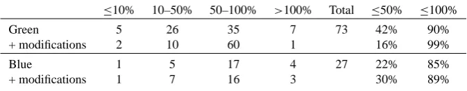
[image:6.595.312.544.64.232.2]Table 1. Distribution of relative errors between the ESR and the ASC measurements of energy fluxes. In every second row the “+ modi-fications” refers to the results from the modified version of the ASC inversion. The last three columns are for the total number of inverted images for each emission line, and the percentage of the events for which the relative error is less than 50% and 100%, respectively.
≤10% 10–50% 50–100% >100% Total ≤50% ≤100%
Green 5 26 35 7 73 42% 90%
+ modifications 2 10 60 1 16% 99%
Blue 1 5 17 4 27 22% 85%
+ modifications 1 7 16 3 30% 89%
26 red images. The inverted all-sky images are composed of 200×200 pixels, which corresponds to an average spatial resolution of 0.9◦pixel. At the location of the ESR beam in the ASC image the grid spacing is slightly denser in lat-itude than in longlat-itude. We averaged the inverted flux val-ues over the nine (spring season 2001) or four (spring season 2002) pixels surrounding the ESR beam position (the grid points may change slightly from season to season if the posi-tion calibraposi-tion of the camera changes). This corresponds to squares of about 6 km by 6 km and about 4.5 km by 4.5 km, respectively. Thus, the area that we average over is much larger than the radar fov of 0.6◦(full width, half power) cor-responding to a circle with a diameter of approximately 1 km at the auroral altitudes. On the other hand, the temporal reso-lution of the ESR data after a 128-s post-integration is much lower than the one of the ASC (20 or 60 s). An extra un-certainty in this comparison comes from the time difference between the ASC and ESR measurements. As the all-sky im-ages are taken every 20 s and the post-integration time of the ESR data is 128 s, these two measurements are usually not exactly simultaneous. For our events, their time separation varies from 0 to 8 s. To minimise this uncertainty, not only the events with a large time difference, but also events with very rapidly varying aurora have been omitted.
Table 1 shows the distribution of the relative errors for green and blue images, with and without the modifications (see Sect. 3.2). The red images did not give good enough results to be compared with the ones from green and blue images (see discussion in Sect. 5). Also included are the to-tal number of the images of both emission lines as well as the percentage of the events, for which the relative error is less than 50% and 100%, respectively.
As the table shows, adding the emission physics modifi-cations makes the otherwise overestimated results from the green images somewhat better by turning more events to smaller energy flux values and thus, smaller errors (see last column of the table). In case of blue images, the effect is similar but the difference is smaller. According to the last column, for both green and blue images the modified inver-sion is better and thus recommended. The actual energy flux values produced by the modified ASC inversion tend to be lower than the Spectrum output, especially as compared to the blue image inversions. This is probably due to the higher spatial resolution of the radar and the fact that the energy
range of Spectrum is not limited at high energies. However, for most of the cases the relative errors are less than 100%, i.e. the energy fluxes obtained from both inversions are the same magnitude.
Taking into account all of the green and blue line ASC im-ages inverted for the radar data comparison (i.e. 73+26=99 images using the modified version of the method), for 35% of them the relative error was less than 50% and for 88% of them less than 100%. In the case of the satellite conjugate events, there were 19 green and blue ASC images inverted in total. Correspondingly, for 36% of them the relative error was less than 50% and for 90% of the cases the error was less than 100%. The error distribution in both the satellite and the radar data comparisons is fairly similar. The modified ASC inversion method tends to slightly underestimate the energy flux values with respect to both the radar and the satellite data: In 63% of the blue images inverted for the satellite events, the ASC inversion results were smaller than the satel-lite measurement, and in 58% of the images inverted for the ESR events the ASC inversion gave smaller values than the Spectrum inversion.
5 Discussion
Fig. 7. A comparison of energy fluxes from blue ASC image along the DMSP satellite trajectory (dotted line) and blue line photometer data along the photometer scan (solid line) of the arc system on 31 January 2001 at 17:08:00 UT. Conversion from the intensity (R) to the energy flux (mW/m2) is done by Eq. (8) and the yield of blue photons of 200 R/(mW/m2).
into account ozone absorption, Rayleigh scattering and some estimates of the aerosol effects (Oikarinen, 2001). However, the inversion does not take into account an enhancement in the blue emission due to the fluorescent scattering at the sun-light part of ionosphere (Lanchester and Rees, 1987). The in-version results based on the red line (630.0 nm) images (not shown) are much less consistent with the measured fluxes than the inverted blue and green line images. The most obvi-ous reasons for the discrepancy are the different altitude pro-files as well as the timing inaccuracy due to the long lifetime of the red emission. In general, the inversion method yields the most accurate electron energy flux in the near zenith re-gion of the image. By using data from two nearby stations the area of reliable inversion results is enlarged. However, if the distance between the two stations is such that the horizon of one fov overlaps with the zenith of the other fov (such as the ABK and MUO stations in the MIRACLE network, see Fig. 1), the less reliable near-horizon data are mixed with the more accurate near-zenith observations and the accuracy of the final results may be deteriorated. This effect should be studied further in the future.
The default spatial resolution of the inversion is 200×200 pixels per image, but it can be increased up to the resolution of the original images, in our case 512×512 pixels per im-age. However, increasing spatial resolution will require more computation time and the size of the output files will grow. We briefly tested the effect of the changing spatial resolu-tion on the inversion results, and the accuracy of the energy flux does not seem to depend much on the spatial resolution of the inversion. Thus, we consider the default resolution as the best option for the statistical studies where the comput-ing time and the size of the output files should be reasonably small.
Other factors that affect the quality of the inversion results may be, for example, weather conditions, moonlight and the image intensifier of the camera. High or thin clouds are of-ten very difficult to distinguish from diffuse or patchy aurora even by a professional observer. Clouds, together with the moon, will be treated as aurora by the inversion and thus overestimate the energy fluxes. Fog or haze may cause the same effect by scattering the moonlight. On the other hand, when the moon is below the horizon and no scattered light is present the cloud cover will diminish the inverted energy flux. However, errors due to these effects are supposed to be minor as compared to the uncertainties in the emission physics, especially because of the careful selection of the events.
In addition to the approximations in the emission physics, uncertainties in the ASC intensity calibration cause some in-accuracy in the results. Calibrating an ASC is a challenging task. For example, the ASCs used in this study have been calibrated with a known light source and a 90◦elevation an-gle only. Although inverting images from several stations together tend to compensate for these uncertainties, other el-evation angles should also be measured in order to obtain a better flat field correction. Furthermore, the combination of fish-eye and telecentric lenses in the ASC optics may lead to some unknown changes in the transmission of the interfero-metric filters. Further complications follow from the fact that the amplification and the stability of the ASC image intensi-fiers depend on their temperature and age.
For our main event on 31 January 2001 (Fig. 1), photome-ter data from Karesuvanto (Kaila and Holma , 2000), which is about halfway between Muonio and Kilpisj¨arvi, were also available. The photometer scanned the triple arc between 17:08:17 UT and 17:08:27 UT. Using Eq. (8) we calculated the energy fluxes from the photometer recordings of the blue emission, as well as from the blue image from the ASC at Muonio (see Fig. 7). Although the photometer scan is not aligned with the satellite trajectory (from which the inversion results are subtracted) and the elevation angle of the measure-ments varies from 35◦to 90◦, the agreement is very good. Thus, at least in this case, the differences between these two ground-based instruments are neglible. In the future, com-parison of larger sets of ASC images to simultaneous pho-tometer recordings will allow us to discuss more about the intensity calibration of these instruments.
wider (from 32 eV to 30 keV) than the one of the inversion method. An integration across the arc measured by the satel-lite gave a field-aligned current of 0.1 A/m, while the corre-sponding value from the modified inversion of the blue and green line image was 0.3 A/m. Although the energy range of the inversion is more limited, it gives an overestimation of the electron number flux (or FAC). According to the DMSP data, a significant part of the energy flux is carried by elec-trons with energies higher than 8 keV. Since the inversion fits the energy flux using its own energy range, the result is an overestimation of the particle flux. Thus, the method gives reliable electron energy flux, but the number flux (or FAC) is good only when the energy flux is carried by the precipitating electrons with energies of 0.1–8 keV.
The characteristic energy of the electron precipitation can be solved as a ratio between the energy and the number flux. The inversion energy range appears to be a problem in this case too. Leaving out the high-energy precipitation (en-ergies over 8 keV) underestimates the electron energy flux, while ignoring the low-energy precipitation (energies below 0.1 keV) underestimates the electron number flux. Conse-quently, the ratio of these fluxes may or may not give rea-sonable mean energy values, depending on the energy char-acteristics at the time, but it cannot be predicted whether or not the average energy obtained from the inversion method is reliable.
6 Conclusions
We have tested the inversion method for all-sky camera im-ages (Janhunen, 2001) and quantified its reliability. The inverted electron energy fluxes were compared both with the low-altitude DMSP satellite and EISCAT Svalbard radar measurements, with and without an option for more ad-vanced emission physics equations. The events for this study were selected from the imaging season 2001–2002 with in-tensity calibrated MIRACLE ASC data. In total we found 4 satellite conjugate events and 73 time instants with nearly simultaneous EISCAT Svalbard Radar recordings. In the case of the satellite conjugate events, the best agreement was found with the energy fluxes inverted from the combination of blue and green all-sky images or blue images alone, when the emission physics modifications (Sergienko and Ivanov, 1993) were turned on, and the satellite crossed the auroral arc at the zenith. In this case, the DMSP satellite measured energy flux peak values of 19.5, 16.0 and 13.0 mW/m2over the triple arc (red curve in Fig. 4). The corresponding es-timates from the inversion method yielded energy fluxes of 19.5, 18.5 and 19.0 mW/m2(turquoise curve in Fig. 4). The results from green ASC images showed an overestimation of the measured flux values. Closer to the horizon of an ASC field-of-view the inverted energy fluxes become less accu-rate due to the low spatial resolution. About 36% of the 19 analysed ASC images showed energy fluxes with rela-tive errors less than 50% with respect to the DMSP satel-lite measurements. In only one case did the relative error
exceed 100%. Despite the fairly different spatial and tem-poral resolutions of the ASC and ESR measurements, the radar conjugate events show that in general the two inversion methods give energy flux values of the same order of magni-tude. For 35% of the images the relative error of the inverted energy flux was less than 50%, for 90% of the images less than 100%. We think that those discrepancies are mainly at-tributable to the aurora being measured in slightly different position and time. With respect to both satellite and the radar data the modified inversion, as applied to blue ASC images, tends to slightly underestimate the measured flux values, but still gives the smallest relative errors. Our best satellite con-jugate event (MUO, 31 January 2001) shows that when the conditions are good, the inversion gives very good agreement with DMSP, as far as the energy flux is compared. The fact that the agreement is also there in other events, although with some scatter of data points, shows that the good agreement of the 31 January 2001 event was not fortuitous.
In summary, we found that the inversion program for ASC images with the emission physics upgrade, produces 2-dimensional energy flux maps that are in quantitative agree-ment with other (pointwise) instruagree-ments. This makes it a useful tool for event-based and statistical studies of the pre-cipitating electron energy flux.
Appendix A Spectrum
The Spectrum program (Kirkwood, 1988) was used to cal-culate the energy fluxes from the electron density profiles measured by the UHF incoherent scatter radar on Svalbard. We used a Matlab version of this program (Olsson et al., 1996). The procedure assumes only one type of precipitation (protons or electrons) and monoenergetic particle beams at each step. It takes into account measurements below 200 km, where the most intense auroral emission occurs. First, an ion-isation rateqi (1/m3s) at the altitudehi is defined as a
func-tion of electron number densityni. The relation between the
ionisation rate and the radar measurementni is
qi =dni/dt+αeffn2i (A1)
where αeff is a model value of an effective recombination
coefficient. The errors due to the modelling ofαeff are of
the order of 30%. The latter term is crucial for stable, diffuse aurora, while the first term dominates in case of more rapidly varying intense aurora. The electron energiesej(keV) giving
the maximum ionisation at the altitudehj can be expressed
as
ej =1.3·(Z(hj)/4.57·10−6)0.57 (A2)
where 1.3 is an empirical factor and Z(hj)is the particle
penetration depth (kg/m2) (Rees, 1963). The next step is to calculate the ionisation rates per unit incident flux (1/m)
Sij =
pj·ej/rj·L(Z(hi)/Rj)·Mx(hi)
eav·Mx(dj)
where pj is the fraction of the energy deposited by
ioni-sation, Rj is the atmospheric depth at the lowest
penetra-tion altitude (kg/m2),rj=Rj/ρj(m),ρjis the mass density
(kg/m3),Lis a function of normalised energy deposition dis-tribution (vs.3in the ASC inversion),dj is the lowest
pen-etration altitude (m), eav is the constant average ionisation
energy of about 35 eV, andMxis the number density of
ion-isable constituents (1/m3). Here,iis the altitude index, and
j the energy index. All the neutral atmospheric parameters (Z,ρ, Mx, R,r) are taken from the MSISE-90 model
at-mosphere. The connection between the ionisation rate and the number flux can be written asqi=Sij ·fj, wherefj is
the differential electron number flux value for the energyej.
The vector form of this equation can be inverted to obtain the differential number flux as f=S−1·q, and finally summed over all energies above 3 keV, to obtain the total energy flux
FE=Pejfj. The energies less than 3 keV would result in
very large uncertainties.
Since the fluxesfj are linear combinations ofqi, we can
estimate the flux uncertainties asdfj=
q P
tij2dqij2 , where
tijare the elements of the inverse matrix S−1. For our events
these uncertainties are about 10%.
Acknowledgements. The work by N. Partamies was supported by the Finnish Graduate School in Space Physics and Astronomy. The MIRACLE network is operated as an international collaboration under the leadership of the Finnish Meteorological Institute. The IMAGE magnetometer data are collected as a Finnish-German-Norwegian-Polish-Russian-Swedish project. EISCAT is an Inter-national Association supported by Finland (SA), France (CNRS), the Federal Republic of Germany (MPG), Japan (NIPR), Norway (NFR), Sweden (NFR) and the United Kingdom (PPARC). The DMSP particle detectors were designed by D. Hardy of AFRL, and data obtained from JHU/APL. We thank D. Hardy, F. Rich, and P. Newell for its use. We also thank Annika Olsson for providing her Matlab version of the Spectrum program. The photometer data were provided by Jouni Jussila from Department of Physical Sciences, the University of Oulu. Finally, we thank Fred Sigernes from the University Centre on Svalbard for providing the Marie Curie fel-lowship for N. Partamies in the beginning of this work.
Topical Editor M. Lester thanks two referees for their help in evaluating this paper.
References
Aikio, A. T., Sergeev, V. A., Shukhtina, M. A., Vagina, L. I., Angelopoulos, V., and Reeves, G. D.: Characteristics of pseu-dobreakups and substorms observed in the ionosphere, at the geosynchronous orbit, and in the midtail, J. Geophys. Res., 104, 12 263–12 287, 1999.
Amm, O.: Direct determination of the Local Ionospheric Hall Con-ductance Distribution from Two-Dimensional Electric and Mag-netic Field Data: Application of the Method using Models of typical Ionospheric Electrodynamic Situations, J. Geophys. Res., 100, 21 473–21 488, 1995.
Amm, O.: Method of characteristics in spherical geometry applied to a Harang-discontinuity situation, Ann. Geophys., 16, 413– 424, 1998.
Amm, O., Janhunen, P., Kauristie, K., Opgenoorth, H. J., Pulkki-nen, T. I., and ViljaPulkki-nen, A.: Mesoscale Ionopheric Electrody-namics Observed with the MIRACLE Network: 1. Analysis of a Pseudobreakup Spiral, J. Geophys. Res., 106, 24 675–24 690, 2001.
Andreeva, E. S., Kunitsyn, V. E., and Tereshchenko, E. D.: Phase difference radiotomography of the ionosphere, Ann. Geophys., 10, 849–855, 1992.
Austen, J. R., Franke, S. J., Liu, C. H., and Yeh, K. C.: Applica-tion of computerized tomography techniques to ionospheric re-search, Radio beacon contribution to the study of ionisation and dynamics of the ionosphere and corrections to geodesy, edited by Tauriainen, A., University of Oulu, Oulu, Finland, Part 1, 25–35, 1986.
Baumjohann, W., Pellinen, R. J., Opgenoorth, H. J., and Nielsen, E.: Joint two-dimensional observations of ground magnetic and ionospheric electric fields associated with auroral zone currents: current systems associated with local auroral break-ups, Planet. Space Sci., 29, 431–447, 1981.
Frey, H. U., Frey, S., Lanchester, B. S., and Kosch, M.: Optical to-mography of the aurora and EISCAT, Ann. Geophys., 16, 1332– 1342, 1998.
Frey, S., Frey, H. U., Carr, D. J., Bauer, O. H., and Haerendel, G.: Auroral emission profiles extracted from three-dimensional re-constructed arcs, J. Geophys. Res., 101, 21 731–21 741, 1996a. Frey, H. U., Frey, S., Bauer, O. H., and Haerendel, G.:
Three-dimensional reconstruction of the auroral arc emission from stereoscopic optical observations, SPIE Proc., 2827, 142–149, 1996b.
Gjerloev, J. W. and Hoffman, R. A.: Height-integrated conductivity in auroral substorms, 1. Data, J. Geophys. Res., 105, 215–226, 2000.
Gustavsson, B.: Tomographic inversion for ALIS noise and resolu-tion, J. Geophys. Res., 103, 26 621–26 632, 1998.
Hallinan, T. J.: Auroral spirals, 2. Theory, J. Geophys. Res., 81, 3959–3965, 1976.
Hardy, D. A., Schmitt, L. K., Gussenhoven, M. S., Marshall, F. J., Yeh, H. C., Schumaker, T. L., Hube, A., and Pantazis, J.: Precip-itating electron and ion detectors (SSJ/4) for the block 5D/flights 6-10 DMSP satellites: Calibration and data presentation, Rep. AFGL-TR-84-0317, Air Force Geophys. Lab., Hanscom Air Force Base, Mass., 1984.
Hedin, A. E.: MSIS-86 thermospheric model, J. Geophys. Res, 92, 4649–4662, 1987.
Hedin, A. E.: Extension of the MSIS thermosphere model into the middle and lower atmosphere, J. Geophys. Res., 96, 1159–1172, 1991.
Janhunen, P., Olsson, A., Amm, O., and Kauristie, K.: Characteris-tics of a stable arc based on FAST and MIRACLE observations, Ann. Geophys., 18, 152–160, 2000.
Janhunen, P.: Reconstruction of electron precipitation characteris-tics from a set of multi-wavelength digital all-sky auroral images, J. Geophys. Res., 106, 18 505–18 516, 2001.
Kaila, K. U. and Holma, H. J.: Absolute calibration of photometer, Phys. Chem. Earth (B), 25, 467–470, 2000.
Kirkwood, S.: SPECTRUM – a computer algorithm to derive the flux-energy spectrum of precipitating particles from EISCAT electron density profiles, IRF Tech. Rep. 034, Swedish Institute of Space Physics, 1988.
Nakamura, R., Baker, D. N., Yamamoto, T., Belian, R. D., Bering, E. A., Benbrook, J. A., and Theal, J. R.: Particle and field signa-tures during pseudobreakup and major expansion onset, J. Geo-phys. Res., 99, 207–222, 1994.
Nygr´en, T., Markkanen, M., Lehtinen, M., and Kaila, K.: Appli-cation of stochastic inversion in auroral tomography, Ann. Geo-phys., 14, 1124–1133, 1996.
Oikarinen, L.: Polarization of light in UV-visible limb radiance measurements, J. Geophys. Res., 106, 1533–1544, 2001. Olsson, A., Persson, M. A. L., Opgenoorth, H., and Kirkwood, S.:
Particle precipitation in auroral breakups and westward traveling surges, J. Geophys. Res., 101, 24 661–24 673, 1996.
Partamies, N., Kauristie, K., Pulkkinen, T. I., and Brittnacher, M.: Statistical study of auroral spirals, J. Geophys. Res., 106, 15 415– 15 428, 2001.
Raymund, T. D., Austen, J. R., Franke, S. J., Liu, C. H., Klobuchar, J. A., and Stalker, J.: Application of computerized tomography to the investigation of ionospheric structures, Radio Sci., 25, 771– 789, 1990.
Rees, M. H.: Auroral ionization and excitation by incident energetic electrons, Planet. Space Sci., 11, 1209–1218, 1963.
Rees, M. H.: Physics and Chemistry of the Upper Atmosphere, Cambridge University Press, New York, 1989.
Rees, M. H. and Luckey, D.: Auroral electron energy derived from ratio of spectroscopic emissions, 1. Model computations, J. Geo-phys. Res., 104, 5181–5186, 1974.
Sergienko, T. I. and Ivanov, V. E.: A new approach to calculate the excitation of atmospheric gases by auroral electron impact, Ann. Geophys., 11, 717–727, 1993.