Minimizing Delay in Network Function
Virtualization with Shared Pipelines
Ori Rottenstreich, Isaac Keslassy, Yoram Revah and Aviran Kadosh
Abstract—Pipelines are widely used to increase throughput in multi-core chips by parallelizing packet processing while relying on virtualization. Typically, each packet type is served by a dedicated pipeline with several cores, each implementing a network service. However, with the increase in the number of packet types and their number of required services, there are not enough cores for pipelines. In this paper, we studypipeline sharing, such that a single pipeline can be used to serve several packet types. Pipeline sharing decreases the needed total number of cores, but typically increases pipeline lengths and therefore packet delays. We consider two novel optimization problems of allocating cores between different packet types such that the average or the worst-case delay is minimized. We study the two problems and suggest optimal algorithms that apply under different assumptions on the input. We also present greedy algorithms for the general case. Last, we examine our solutions on synthetic examples as well as on real-life applications and demonstrate that they often achieve close-to-optimal delays.
Index Terms—Multicore Optimization, Network Function Vir-tualization, Network Processors.
I. INTRODUCTION
A. Background
This paper introduces the novel problem ofpipeline sharing, which designers face when implementing the emerging class of dedicated pipeline-based multi-core chips. This group encom-passes multi-core network processors [2], [3], and application-specific systems-on-chip (AS-SoC) such as telecommunication applications [4] and high-end multiprocessors [5]. Recently, NFV (Network Function Virtualization) was described as a new networking framework. It suggests to implement various network functions in identical virtual machines by relying on virtualization [6]. Practically, such virtualization must consider restrictions on the number of available cores.
Consider a set of numbered services, and a flow of incoming packets, where each packet may need to go through a different subset of services in an increasing order. Dedicated chips used to be implemented with a single general-purpose core that could provide all the needed services using software-based algorithms. However, such a single software-software-based core would not be scalable. Therefore, dedicated chips have become implemented asmulti-corechips, where each core (or engine) is specifically designed to implement asingleneeded service.
This manuscript is an extended version of “Minimizing Delay in Shared Pipelines”, which was presented in IEEE Hot Interconnects ’13, San Jose, CA, USA, August 2013 [1].
O. Rottenstreich is with Princeton University, NJ, USA (email: [email protected]). I. Keslassy is with VMware, CA, USA and the Technion, Israel (e-mail: [email protected]). Y. Revah and A. Kadosh are with Marvell, Israel (e-mails:{yoramr, aviran}@marvell.com).
Deep packet inspec,on
Packet type 1
Delay = 3 Ingress ACL Rou,ng modifica,on Header
Packet type 2
Delay = 2 Bridging Rou,ng
Packet type 3
Delay = 3 Rou,ng modifica,on Header
(a) Three pipelines with 8 cores (without pipeline sharing). The average delay isT ≈2.67time slots and the worst-case delay isD= 3time slots.
Deep packet inspec,on Packet type 1,3
Delay = 4 Ingress ACL Rou,ng modifica,on Header
Packet type 2
Delay = 2 Bridging Rou,ng
[image:1.612.322.508.182.282.2](b) Example of pipeline sharing: Two pipelines with only 6 cores. The average delay isT ≈3.33time slots and the worst-case delay isD= 4time slots.
Fig. 1. Illustration ofpipeline sharing.
Thus, each packet could go through all the corresponding cores to obtain all its needed services.
Letting packets go through their needed cores one after another would result in unpredictable queueing delays, and therefore a lack of performance guarantees. Hence, an appeal-ing solution is to usepipelines. Assume that packets are divided into k differentpacket types, where each packet type needs a specific set of services. Then, the chip can be implemented using exactlykpipelines, where the pipeline that corresponds to each packet type includes the cores that implement its needed services. Incoming packets are simply forwarded to their appropriate pipelines. If at most one packet arrives every time slot, and each core processing takes one time slot, then it is guaranteed that each packet will be done with processing in the minimal needed time, without any potential conflict on its processing path.
after a number of time slots that equals the number of cores in its pipeline. If thek packet types are uniformly distributed, the obtained average delay is(3 + 2 + 3)/3≈2.67time slots. Likewise, the worst-case (maximal) delay, is 3.
However, following the increase in (a) the number of packet types, and (b) the pipeline lengths, the number of needed cores does not fit multi-core chips anymore. Therefore, we need to rely onpipeline sharing, such that different packet types may need to go through the same pipeline. As a result, a pipeline may include more services than needed by a packet. When a packet encounters a core that it does not need, it simply does not use it, but still spends time in it in order not to break the pipeline. Therefore, while pipeline sharing decreases the needed number of cores, it can also increase the packet delay. Fig. 1(b) illustrates this pipeline sharing. The first and the third packet types share the first pipeline, which includes the 4 cores required by at least one of these types. Hence, we only need6cores instead of 8. On the other hand, since these two types now require a larger delay of 4 time slots to go through their shared pipeline, the average delay increases to
(4 + 2 + 4)/3≈3.33and the worst-case delay is now 4 instead of 3.
For a minimal implementation cost, the design assumes a very simple control logic which basically maps an incoming packet to the corresponding pipeline. Such a simple control logic does not support skipping pipeline steps, early pipeline termination or allowing packets to cross several pipelines.
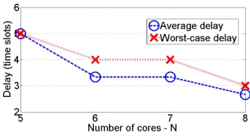
There is a clear tradeoff between the number of needed cores and the obtained average and worst-case packet delays. This tradeoff creates capacity regions in the design exploration, in the sense that the minimal possible delay is described for a given upper bound on the number of cores. A designer cannot go below these optimal bounds. This is illustrated in Fig. 2. For instance, with at most5cores a single pipeline must serve the three packet types with 5distinct services and result in an average delay and worst-case delay that both equal5. Likewise, allowing the existence of a seventh core cannot improve the optimal delays that can be obtained with at most6cores. The goal of this paper is to further analyze these optimality bounds. In this paper we introduce pipeline sharing in multi-core chips. A limited number of cores should be divided into pipelines, each serving several packet types. To minimize the delay of a packet we try reduce the lengths of these pipelines.
B. Related Work
Several past works have considered the problem of mapping the pipelines onto the chip cores in order to reduce energy consumption and bandwidth utilization [7]–[9]. These mapping issues are outside the scope of the paper, and the mapping solutions are complementary to our suggested algorithms, in the sense that they can be applied on the resulting pipelines.
[image:2.612.347.528.54.153.2]Pipeline scheduling was discussed in [10]. This work deals with a simpler problem in which the hardware components are not configurable and each of them can perform a single predetermined task. For instance, given a formula with several additions and multiplications, they study how to schedule simultaneously several pipelines calculating the formula. They
Fig. 2. Tradeoff between the number of cores and the average or worst-case delays, defining capacity regions for the two optimization problems. For a limited number of cores, the minimal possible delays are presented. A designer cannot go below these optimal bounds.
try to guarantee that in every time unit a single adder and a single multiplier are not used by more than a single pipeline.
The design of multicore systems was discussed for a wider range of environments besides pipelines. [11] analyzed the number of cores that should implement each task based on its utilization. [12] studied the obtained system throughput as a function of the partition granularity of the different requirements into small tasks. Finer granularity can improve the performance but also complicates the mapping process.
In addition, network processors (NPs) may adopt additional alternative architectural models. For instance, the multipass NP architectural model is suggested in [13] as an alternative to pipelining. While such a model may have less synchroniza-tion issues than pipeline-based models, it may also provide fewer guarantees of service. A multi-queued NP architecture was suggested in [14] to serve packets with heterogeneous requirements. They study a policy that may omit a packet upon the arrival of a second packet with simpler requirements.
Our problem can also be viewed in the context of recent ongoing research on NFV, including function assignment opti-mization [15]. Consequences from our work can be useful also in this framework, e.g. by deciding how many cores should implement every function or what flows to serve by the same pipeline.
II. MODEL ANDPROBLEMDEFINITION
We start by introducing notations and formally defining the problems discussed in this paper.
A. Traffic
We consider a system where each packet needs to perform a set of required tasks amongrpossible tasks,{1,· · ·, r}. Each task is performed exactly once for each packet, in an increasing index order. For instance, out ofr= 10possible tasks, a packet may need to perform tasks {1,2,7}. It will successively run tasks 1, then 2, and finally 7.
We further assume that there are k types of packets. Each incoming packet has a probabilitypi >0 of belonging to type i, and packets of type ineeds to perform a fixed set of tasks
Si. For instance, an incoming packet may either be of type1 with probabilityp1 = 0.6 and require tasksS1={1,2,3}; or it may be of type2with probabilityp2= 0.4and require tasks
Our analysis and solution are not sensitive to whether each packet of type i appears with probability pi independently of its preceding packets or whether there are some dependencies between subsequent packets (e.g., the existence of long flows with several packets of the same type) that yield a stationary distribution with these probabilities.
We restrict the model to consider tasks that can be ordered as above. Clearly, in some systems two tasks might be required in different orders by two packets and our study does not cover them. Notice that it is impossible to share two pipelines, al-though they include the exact set of tasks if the required orders of one or more pairs of tasks are different. We take advantage of this restriction to enable improved performance by being able to share more pipelines. Indeed, this possibility to order tasks is common for different networking systems. A recent study [16] surveyed a wide range of middlebox applications. It describes the implementation of each application as an ordered list of processing steps. They name 10 processing steps in a specific order such that each application is associated with a subset of them according to the common order. Earlier, a methodology to profile multiprocessor and network processor applications by representing them as directed acyclic graphs (DAG) was described [17], [18]. In this representation, nodes represent computational tasks and links represent control and data dependencies. Various types might require similar variants of the application with part of the tasks, described as a path in the graph. While the graph might enable degrees of freedom in ordering the tasks, for any such DAG, our model can be applied by selecting an arbitrary legal order. The pipeline sharing performance is not affected by this selection.
Another application can be found in a simplified version of the compilation of programming languages for packet for-warding architectures such as the recently developed popular language P4 [19]. In its compilation, a DAG is used to de-scribe dependencies between logical tables, each implementing a computation task. Assuming equal-size tables of a single matching type, this translation can follow the model while trying to implement these computation tasks by processing cores.
Some applications can benefit from having more than a single possible service path for the same packet type. Our model gives higher priority to the reduction of the delay rather than maintaining the flexibility. Keeping the cores required for that for one flow decreases the core availability for other flows and can enforce unnecessary pipeline sharing with an increased delay.
B. Pipeline Sharing
We are now interested in studying how the set of cores in a multi-core chip can be subdivided into shared pipelines that can service the different packets.
We assume that the chip holds N cores. Each core is an homogeneous general-purpose core that can be configured to serve any task. By relying on virtualization, at run-time, the chip manager configures each of the cores to serve a single task among the set of possible tasks, e.g. by loading it with a different code. Due to limitations on its memory size, the
core cannot be configured to serve two or more tasks. The chip manager further subdivides the N cores into d pipelines of multiple separate cores. Let Qi be the set of tasks served by the ith pipeline.
For example, a chip withN = 9cores could be subdivided into one pipeline of 2 cores that respectively deals with tasks1
and2; another pipeline of 3 cores that processes tasks 1,2,3; and another pipeline of 4 cores that deals with tasks1,3,4,5. Note that each of the three pipelines holds a separate core that processes task 1, i.e. several cores may be assigned the same task.
In addition, the chip manager assigns a single pipeline to each packet type, such that the pipeline contains all the tasks required by this packet type. For instance, it may assign packets of type 2 that needs the set of tasks S2 = {1,4} to the last pipeline of cores, which processes tasks1,3,4,5. In this case, note that the packets will just go through the cores of tasks 3 and 5 without any processing.
C. Optimization Problems
We model the delay of a pipeline as equal to its length, i.e. its number of cores. In our example, it will take 4 time-slots to go through the pipeline of 4 cores that processes tasks1,3,4,5. So if a packet that needs the task setS2={1,4}goes through this pipeline, it will still take 4 time-slots, out of which the two slots for processing tasks 1 and 4 are useful, while the two other slots are simply empty. Early pipeline termination is not allowed and a packet cannot leave the pipeline before reaching its last core due to the limited control of the system. Thus, there is a clear tradeoff between the flexibility of a longer pipeline, which can process more packet types, and its higher delay.Given our set ofN cores, our goal is to use this tradeoff in order to reduce the average or the worst-case packet delay.
Formally, we state our first problem as follows: Given N
cores, and the ksets of tasksSi of probabilitypi,our goal is to find shared pipelines that will minimize the average packet delay. We denote byTOP T(N)this minimal possible average delay.
Likewise, in our second problem, givenN cores and the k
sets of tasks Si of probability pi, our goal is to find shared pipelines that will minimize the worst-case packet delay. We denote byDOP T(N)this minimal possible worst-case delay.
Note that we use the term packet for the item served in the pipelines. While this is especially relevant for network processors, in other pipeline architectures the more general term ofelement is also very common.
D. General Properties
avoid having pipelines that include both security and traffic shaping tasks. The importance of this property is by helping us, later in this paper, to find optimal solutions for families of instances of the problems.
Proposition 1. Assume that thertasks can be divided into two categories such that each type requires tasks from one category, i.e. the kpacket types can be ordered such that
Sm
i=1Si
∩
Sk
i=(m+1)Si
=∅for somem∈[1, k]. Then, for each of the problems, an optimal solution givenN cores can be obtained for some value N0 ∈ [0, N] as the union of the pipelines in optimal solutions for packet types[1, m]and for types [(m+ 1), k] withN0 and(N−N0)cores, respectively.
Proof: Consider a pipeline in an optimal solution that serves tasks from both setsSm
i=1Si
,Sk
i=(m+1)Si
. Then, it can be partitioned into two smaller pipelines to reduce the average delay without increasing the worst-case delay. Ac-cordingly, we can distinguish between pipelines in an optimal solution according to the category of tasks they serve.
Similarly, the next proposition shows that if the sets of tasks (for the different packet types) served by a pipeline can be divided into two disjoint unions of tasks, then this pipeline can be divided into two shorter pipelines which will result in a shorter average delay and at most the same worst-case delay. The proof is similar to the last one and is omitted for its simplicity.
Proposition 2. Let Si1,· · · , Sib be the sets of tasks served by one of the pipelines in a solution for one the two problems. If for somem∈[1, b]we haveSm
j=1Sij
∩Sb
j=(m+1)Sij
=
∅ then the pipeline can be divided into two pipelines without increasing the number of cores. This results in a shorter average delay and at most the same worst-case delay.
III. MINIMIZING AVERAGE DELAY
In this section, we study our first optimization problem of minimizing the average delay. We present an optimal algorithm that applies when the input satisfies a specific property, describe some general properties of the problem, and provide a greedy algorithm for the general case.
A. A simple case of the required tasks:Si= [1, Yi]
Finding an optimal solution of the problem that minimizes the average delay is difficult in the general case. Here, we consider a property of the sets of tasks required by the different packet types S1,· · ·, Sk that when satisfied allows us to efficiently calculate an optimal solution that minimizes the average delay.
In some applications all packet types demand several con-secutive tasks starting from the first task. The different packet types differ in the number of required tasks in each of them. Then, the set of tasks of packet type i can be presented as
Si={1,· · ·, Yi}= [1, Yi]for Yi∈[1, r].
For instance, this scenario can describe a required packet processing hierarchy for packets with different required levels of security. If an Intrusion Detection System (IDS) service is
partitioned into smaller tasks in which disjoint pattern sets are examined, a packet with a higher security level might require to be compared with a larger set of patterns. This can be described as additional tasks required by the packet. In particular, the Snort IDS [20] defines the notion of severity level. It enables customizable prioritization of alerts such that the severity level of 32 predefined alert categories can be modified. Then, the highest priority alerts (with lowest severity levels) are examined by installing corresponding rules of all categories with up to some specific severity level. A task can be described as examining the rules of one level such that different packet types would require running different number of the first tasks.
We show that in such cases an optimal solution has several properties such as specific forms of its pipelines as well as simplicity in the matching of the packet types to one of the pipelines. These properties enable us to suggest an efficient algorithm for finding an optimal solution.
In the rest of the section, we assume that S1 =
[1, Y1],· · · , Sk= [1, Yk]⊆[1, r]are ordered such thatYa≤Yb
if a < b. We then have that S1 ⊆ S2 ⊆ · · · ⊆ Sk−1 ⊆ Sk.
Indeed, by merging identical requirements, the set of tasks can be ordered such thatS1,· · ·, Sk satisfy the required condition whenever S1 ⊆S2 ⊆ · · · ⊆Sk−1 ⊆ Sk. Let Q1,· · ·, Qd be the set of tasks serviced by the cores in the dpipelines in an optimal solution and let (B1,· · · , Bk) be a vector indicating the serving pipeline for each packet type s.t. Bi ∈ [1, d]. For short, we denote the range[1,1]by[1].
The properties are summarized in the following lemmas. The first lemma explains that the cores in a pipeline should be those required by the packet type with the largest set of tasks among the types it serves.
Lemma 1. The pipelines in an optimal solution Q1,· · ·, Qd satisfy for j∈[1, d] Qj ∈ {S1,· · · , Sk}, i.e. the sets of tasks in the pipelines in an optimal solution are among the sets of tasks of the different packet types in the input. In particular, for j∈[1, d]Qj is of the formQj = [1, Zj] for Zj∈[1, r].
Proof: Let h be the number of packet types served by pipelineQjand letSi1, Si2,· · · , Sih−1, Sihbe the sets of tasks
of these packet types such that i1 < i2 <· · · < ih−1 < ih. According to the order of S1,· · ·, Sk, we have that Si1 ⊆ Si2 ⊆ · · · ⊆Sih−1 ⊆Sih. By the correctness of the solution,
we have thatSh
m=1Sim ⊆Qj. In addition, by the optimality
of the solution, an equality must hold i.e. Sh
m=1Sim = Qj.
Otherwise, cores could be eliminated to reduce the delay. Since
Si = [1, Yi]it follows that Qj =S h
m=1Sim =Sih = [1, Yih].
The next lemma presents a property of the matching of packet types to pipelines in an optimal solution.
Lemma 2. Assume that Q1,· · ·, Qd are ordered such that Q1 $ Q2 $ · · · $ Qd−1 $ Qd. Then, the packet types are served by an increasing order of the pipelines, i.e. Bi ≤Bj
fori < j. In particular, the packet types served by each pipeline
in the solution form a subset of consecutive packet types. In particular, the last packet type is served by the last pipeline, i.e. thekth packet type is served by Q
Bk=Qd=Sk.
Algorithm 1 Optimal Algorithm for Minimizing the Average Delay for Si= [1, Yi](Pseudo-code)
Input:
1 Packet types with sets of tasks S1 = [1, Y1],· · ·, Sk =
[1, Yk] and probabilitiesp1,· · ·pk.
2 Initialize: Forn≥0: T(0, n) = 0. Forn <0: T(0, n) =
∞. Fori >0, n≤0:T(i, n) =∞. Forn≥0:B(0, n) = () (an empty vector) and Q(0, n) = {} (an empty set of pipelines).
3 Main:
4 fori= 1 tokdo
5 forn= 0 toN do
6 Calculate T(i, n)according to Eq. (1) 7 Calculate Q(i, n)according to Eq. (2) 8 Calculate B(i, n) according to Eq. (3)
9 returnQ(k, N),B(k, N)
to Lemma 1. Assume that the claim does not hold for an optimal solution and let i, j be two indices such that i < j
and Bi > Bj. Then, based on the order of S1,· · · , Sk and
the correctness of the solution Si⊆Sj ⊆QBj $QBi and in
particularSi⊆QBj. We can let packet typeibe served byQBj
that satisfies|QBj|<|QBi|and reduce the average delay of the
solution in contradiction to its optimality. In addition, with the last property if Bi =Bj (for i < j) then Bm=Bi=Bj for allm∈[i, j]and every pipeline serves a subset of consecutive packet types.
Following this lemma, we suggest a dynamic-programming algorithm to find an optimal solution to this special case of the problem. To do so, we suggest several additional definitions. We denote by T(i, n) (for i∈[0, k],n∈[0, N]) the minimal possible weighted average delay that can be achieved in serving the firstipacket types given at mostncores. In the calculation of this average we consider each of thei packet types with a weight that is equal to its original probability such that for
i < k the sum of weights is smaller than one. If no such
solution exists we define T(i, n) = ∞. We later explain that the optimal average delayTOP T(N)equalsT(k, N). Likewise, we denote by B(i, n) (for the same values of i, n whenever
T(i, n) 6= ∞) the vector of length i that indicates for each packet type the serving pipeline in an optimal solution for the firstipacket types with at mostncores. Last, letQ(i, n)denote the list of pipelines in this optimal solution. This list is ordered as assumed in Lemma 2. The next example demonstrates these definitions.
Example 1. Assume an input of k = 3, N =
8 and (S1, p1),(S2, p2),(S3, p3) = ([1],0.3),([1,3],0.2),
([1,5],0.5). With at most three cores, for instance, we can serve the first type with a pipeline of a single core and thus T(1,3) = 0.3. Likewise, we can serve the first two types by a pipeline of three cores that results in a delay of three for these two types and accordingly,T(2,3) = (0.3 + 0.2)·3 = 1.5. For this input, an optimal solution with at most N = 8 cores is composed of two pipelinesQ(k, N) =Q(3,8) ={[1],[1,5]}in which the first type is served in the first pipeline in the solution
[1] = {1} while the second and third type are served by the second pipeline [1,5] = {1,2,3,4,5}. This is represented by B(k, N) =B(3,8) = (1,2,2). This result in an optimal delay T(k, N) =T(3,8) = 0.3·1 + (0.2 + 0.5)·5 = 3.8. To serve the three types given at most8cores, we have several options that differ in the number of additional types that are served with the last type in the pipeline of 5 cores. Three cores are left for the other pipelines. This can be either only the last type itself (with probability of 0.5) or the second type together with the third (with probability of 0.2 + 0.5 = 0.7) or all the three types (with probability of 1). Accordingly, T(k, N) = T(3,8) = min (T(2,3) + 0.5·5, T(1,3) + 0.7·5, T(0,3) + 1·5).
We present recursive formulas for the functions
T(i, n), Q(i, n) and B(i, n) based on the idea from the example. For the correctness of the following recursive formulas, we set T(0, n) = 0 for n ≥ 0, T(0, n) = ∞ for
n <0 andT(i, n) =∞ fori >0, n≤0. Likewise, forn≥0
we setB(0, n) = () (an empty vector) andQ(0, n) ={} (an empty set of pipelines).
The intuition behind the formulas is the following. To calculateT(i, n), we consider an optimal solution for the first
i packet types. By Lemma 2, the ith packet type (S
i, pi) is served by the last pipelineQBi =Si and has a delay of|Si|.
Additional packet types may be served by this pipeline. If we denote the total number of packets served by this pipeline byj, thenj∈[1, i]and by the same lemma, we must have that these are the packet types with indices [i−(j−1), i]. To calculate the minimal delay, we consider the best option for the value of j from the above values. Since |Si| cores are used by the last pipeline, the first (i−j) packet types can be served by the other (n− |Si|) available cores. Their minimal possible contribution to the average delay is T(i−j, n− |Si|) and it can be achieved according to an optimal solution for these parameters. To calculate Q(i, n) and B(i, n) we look at the possible identities of the pipelines in such a solution. If there exists a solution withjpacket types served by the last pipeline, we add to the pipelines in an optimal solution of the firsti−j
packet types, an additional single pipeline ofSi. The vectorB is now updated such that the last j packets are served by the last pipeline with an index of |Q(i, n)|. Based on the above, we can deduce the following.
Theorem 1. (i)Fori∈[1, k], the variableT(i, n)satisfies
T(i, n) = min
j∈[1,i] T(i−j, n− |Si|) +
i
X
m=(i−(j−1))
pm
!
· |Si|
!
(1)
(ii)Letjbe the minimal value of the corresponding parameter that minimizes the right-hand side of (i). Then, there exists an optimal solution that satisfies
Q(i, n) =Q(i−j, n− |Si|)∪ {Si}, and (2)
B(i, n) =B(i−j, n− |Si|)·(|Q(i, n)|,· · ·,|Q(i, n)|)
| {z }
jtimes
(3)
Finally, we describe the suggested dynamic-programming algorithm. Its pseudo-code is presented in Algorithm 1. We first initialize T(0, n) = 0 for n ≥ 0, T(0, n) = ∞ for
n < 0, T(i, n) = ∞ if i > 0 and n ≤ 0, B(0, n) = ()
andQ(0, n) ={}forn≥0 (line 2). We continue to calculate in step i (for i ∈ [1, k]) the values ofT(i, n)for n∈ [0, N]
according to the formulas presented in Theorem 1 based on the values from previous steps (lines 4-8). In the required solution, all thekpacket types have to be served withNavailable cores. Thus the optimal average delayTOP T(N), the pipelines in an optimal solution and the matching of packet types to pipelines are given by T(k, N), Q(k, N)andB(k, N), respectively.
We now discuss the time complexity of the suggested algorithm. The algorithm is composed ofksteps, in each step
i ∈ [1, k] we calculate the (N + 1) values of optimal delays
T(i, n) for n∈[0, N]. For each value, by relying on Eq. (1) from Theorem 1, we take the minimal value out of at most k
possible values (line 6, according to the maximal value ofiin this equation) or perform more simple calculations (lines 7-8). Thus the time complexity isO(k2·N). The representation of
Q(i, n)for somei, nincludes at mostkpipelines with a length that equals at most the number of distinct possible tasksr. The algorithm keepsQ(i, n)forkvalues of the first parameter and for (N+ 1) values of the second. The memory required for storing one value of T(i, n), B(i, n) is smaller. The memory complexity of the algorithm is accordinglyO(k2·N·r).
B. General Properties
We now describe some basic properties of this problem of minimizing the average delay. These properties can be used by a designer to understand the limits of the chip design capacity region. The simple proof of the first of them is omitted due to space limits.
The first property discusses the value of the optimal delay as a function of the number of cores. Intuitively, for a too small number, we cannot serve some the tasks and for a large enough number, each type can have a dedicated pipeline.
Proposition 1. (i) For all N ≥0, the optimal average delay is at least as large as the (weighted) average size of a set of tasks, i.e.TOP T(N)≥P
k i=1
pi· |Si|
.
(ii) TOP T(N) =P k i=1
pi· |Si|
forN ≥Pk i=1|Si|. (iii)The number of cores should be at least the number of dis-tinct tasks in the input, i.e.TOP T(N) =∞forN <|Ski=1Si|. The next property presents a condition that must be satisfied for every packet in an optimal solution.
Proposition 2. In any optimal solution (i.e. a solution with a delay ofTOP T(N)), every packet type is served by a pipeline that has the minimal length among the pipelines that serve all the tasks of the packet type.
Proof:Clearly, if this is not the case for one of the packet types, we can let this packet type be served by an existing pipeline with shorter length and reduce the average delay.
C. Pipeline Merging Algorithm for Minimizing the Average Delay
We suggest an efficient greedy algorithm for reducing the average packet delay for a general input. Intuitively, it can be efficient to serve within the same pipeline several packet types with a large number of common tasks, so that their merging would result in a small delay increment. The algorithm starts with an initial state in which there is a pipeline for each of the packet types. This initial state would need many cores to be implemented, and would typically exceed the number of available cores on the multi-core chip. Therefore, our algorithm iteratively reduces the number of needed cores. Specifically, at each iteration, itmergestwo of the remaining pipelines into a single shared pipeline. It only ends when the merged pipelines can finally be implemented using the multi-core chip (or when there is clearly no solution).
In other words, consider a given iteration of the algorithm. Assume that its pipelines currently usencores. Ifn≤N, the pipelines can be implemented and the current state is returned as the solution. Else, we select two pipelines and merge them. Then, packet types that make use of these pipelines might observe a larger delay after this operation.
For a given pair of pipelines, letxbe the increment in the average delay if these pipelines are merged. Further let y be the corresponding decreased number of cores. Intuitively, it is better to merge a pair of pipelines with a small ratiox/y.
We calculate x, y for every pair of pipelines. Let Ai (for i∈[1,2]) be the set of cores in each of the two pipelines of the pair. This set of cores is the union of the cores required by the packet types served by this pipeline. Likewise, letzibe the probability of an arbitrary packet to belong to a packet type served by this pipeline. This is the sum of the probabilities for a packet to belong to one of the packet types served by the merged pipeline.
We consider only meaningful pairs of pipelines, i.e. pairs with common cores. Merging pipelines with disjoint sets of cores cannot reduce the number of cores. For these valid pairs, we examine the three following criteria. (a) Large number of common cores, (b) Small number of non-common cores, and (c) Low probability for an arbitrary packet to belong to a type served by the merged pipelines.
The additional delay for packets previously served by the first pipeline (fraction of z1 of all packets) is |A2 \ A1|. Likewise, for packets served by the second pipeline (z2 of all packets) the additional delay is |A1 \A2|. Thus the in-crease in the average delay if these pipelines are merged is
x=z1· |A2\A1|+z2· |A1\A2|. This is thecost. If the two pipelines in the pair are merged, the total number of cores is reduced by the number of common coresy=|A1∩A2|>0. This is thegainin such merging.
For this pair, we define the ratioRas the marginal cost, i.e.
R=x/y= (z1· |A2\A1|+z2· |A1\A2|)/|A1∩A2|. In each step of the algorithm we simply merge the pair of pipelines with the minimal marginal cost.
that in this algorithm, keeping the current set of pipelines is required only for the last outer loop. Other variables require a smaller amount of memory. Thus the memory complexity is
O(k·r).
Example 2. Consider again the input from Example 1 with k = 3, N = 8 and (S1, p1),(S2, p2),(S3, p3) =
([1],0.3),([1,3],0.2), ([1,5],0.5). For i, j ∈ [1,3], let Ri,j be the value of the ratio R as defined above for the pair of packet types(Si, pi)and(Sj, pj). Here, R1,2=(0.3·2 + 0.2·
0)/1 = 0.6, R1,3 = (0.3·4 + 0.5·0)/1 = 1.2 and R2,3 =
(0.2·2+0.5·0)/3≈0.133. Since the minimal ratio isR2,3, the suggested algorithm merges the second and third pipelines. We then obtain a solution with two pipelinesQ1= [1], Q2= [1,5] which is the optimal solution for this input.
In Section VI, we show experiments for which the suggested (greedy) algorithm results in a delay that often equals (or is very close), to the minimal possible delay. However, as demon-strated in these simulations, the algorithm is not necessarily optimal.
IV. MINIMIZING WORST-CASE DELAY
In this section, we consider a new objective function of min-imizingthe worst-case delay, i.e. the maximal delay obtained by one of the packet types. Here, given a limited number of cores N, a set of k packet types S1,· · ·, Sk (with positive probabilities p1,· · ·, pk > 0), we are looking for shared pipelines that minimize the worst-case delay of all packet types, i.e. the maximal length of a pipeline. We denote byDOP T(N) the minimal possible worst-case delay as a function of the number of cores.
A. General Properties
Our first observation is that a solution that minimizes the average delay does not necessarily minimizes also the worst-case delay. It is illustrated in the following example.
Example 3. Letk= 3, N= 6 and (S1, p1),(S2, p2),(S3, p3) = ({1,2,3},0.2),({3,4},0.2), ({4,5},0.6). To minimize the average delay, it is better to merge the first two pipelines of types with smaller probabilities obtaining pipelines Q1,1 =
{1,2,3,4}, Q1,2 = {4,5} with average delay T1 = 0.4 ·
4 + 0.6 · 2 = 2.8 and worst-case delay of D1 = 4. To minimize the worst-case delay, it is better to merge the two last shorter pipelines obtaining two pipelines of length 3, Q2,1 = {1,2,3}, Q2,2 = {3,4,5} with average delay and worst-case delay that both equalT2=D2= 3.
Another immediate observation is the independence of
DOP T(N)of the exact values of the positive probabilities of the packet types p1, . . . , pk. That is because the optimization function depends on the length of the longest pipeline regard-less of any of the probabilities. Likewise, any of the constraints on a legal solution does not involve these probabilities. Accord-ingly, in this section we will characterize a packet type simply by its required set of tasksSi.
We now describe some basic properties of this new problem, considering the worst-case delay. Next we present bounds on
this delay as a function of the number of cores N. As in the case of the average delay, these bounds can be helpful for a designer to understand the dependence ofDOP T(N)on N. Proposition 1. (i) For all N ≥ 0, DOP T(N) = ∞ or DOP T(N) ∈ {1,2,· · · , r}, namely whenever the worst-case delay is finite, it has an integer value of at mostr.
(ii) For all N ≥ 0, the optimal worst-case delay is at least as large as the optimal average delay, i.e. DOP T(N) ≥
dTOP T(N)e.
(iii) For all N ≥ 0, the optimal worst-case delay is at least as large as the size of the largest set of tasks in the input, i.e. DOP T(N)satisfiesDOP T(N)≥maxi∈[1,k]|Si|.
(iv)For a large enough number of cores, the worst-case delay exactly equals the size of the largest set of tasks in the input, i.e.DOP T(N) = maxi∈[1,k]|Si| forN ≥P
k i=1|Si|.
(v)The number of cores should be at least the number of dis-tinct tasks in the input, i.e.DOP T(N)satisfiesDOP T(N) =∞
for N <|Sk
i=1Si|.
Proof: Whenever all packet types are served, the worst-case delay is the delay of the longest pipeline in the solution. The solution is of course composed of pipelines with an integer number of cores. The length of each pipeline equals at most the number of possible tasks r. In addition, the length of the longest pipeline is clearly not shorter than the (weighted) average length of the pipelines. In any solution a packet type with a set of tasksSi is served by a pipeline Qj that satisfies Si ⊆ Qj. The delay |Qj| that the packet type encounters equals |Qj| ≥ |Si| and the worst-case delay among all the k packet types must satisfy DOP T(N)≥maxi∈[1,k]|Si|. For a large enough number of cores (satisfying N ≥Pk
i=1|Si|), each packet type Si is served separately by a pipeline of length |Si| and the worst-case delay is simply DOP T(N) =
maxi∈[1,k]|Si|. Last, since each of the|S k
i=1Si|distinct tasks must be implemented by a dedicated core, any legal solution cannot be found wheneverN <|Sk
i=1Si|.
We now shortly consider the simple case of S1,· · · , Sk described in Section III-A, for which the sets of required tasks are of the formSi={1,· · · , Yi}= [1, Yi]for Yi ∈[1, r]. It is easy to see that for this case an optimal solution for the worst-case delay is simply given by a single pipeline with the cores required by the largest set in the input. Clearly, any solution that serves all packet types requires at least that number of cores and entails such a delay.
We present additional properties of an optimal solution that minimizes the worst-case delay for a general input. The fol-lowing property is useful to decrease the algorithm complexity, and will be used in Section VI of simulations. Intuitively, with regard to the worst-case, a packet type with a set of tasks Si can always be served by a pipeline that serves a packet type with a setSj that is a super set ofSi.
for the inputS1,· · ·, Sk (with the same value of the parameter N). In extending this solution, by simply serving each pipeline in Si ∈ {S1,· · · , Sm} using the pipeline that serves Sj ∈
{Sm+1,· · ·, Sk} s.t. Si ⊆Sj, we can obtain a solution that achievesDOP T(N).
Proof: By considering the sets of tasksSm+1,· · ·, Sk, a subset of the original sets of tasks, the optimal solution has a delay D≤DOP T(N). Namely, this delay cannot be longer than the optimal delayDOP T(N)for the larger setS1,· · ·, Sk. By serving each of typeSi∈ {S1,· · ·, Sm}by a pipeline that serves typeSjs.t.Si⊆Sj, the set of pipelines in the solution is not changed and the same delayD satisfyingD≤DOP T(N) is obtained for the original input. Thus, clearlyD=DOP T(N) and the set of pipelines is optimal also forS1,· · ·, Sk.
B. A simple case of the required tasks:Si= [Xi, Yi]
We discussed earlier a simple case of the input for which a solution achieving an optimal average delay can be found. We now present an algorithm that achieves the optimal worst-case delay for a generalized class of possible inputs. The algorithm applies when the sets of required tasks are all of the form of ranges, namely each set includes some consecutive tasks and for i∈[1, k] the setSi is of the formSi = [Xi, Yi]. Clearly, this case generalizes the set of legal inputs discussed earlier of the formSi= [Xi, Yi].
This case is applicable for instance in a network in which a task is associated with a network layer in which it is served, e.g.traffic segmentationanderror correctionat layer 2,routing
at layer 3 orload balancingat layer 7. If a packet type requires the tasks of several consecutive layers (for instance, the tasks of layers 2-4), the demands of the different packets can be presented in the above form by simply ordering each task according to the layer it belongs to.
Based on Lemma 1, we also assume that none of the ranges is fully contained in another range. If this is the case for some of the ranges, we could ignore them while trying to find the optimal solution. In addition, we assume that these k sets of tasksS1= [X1, Y1],· · · , Sk = [Xk, Yk]are ordered in an non-decreasing order of the first value in each range, i.e.Xi≤Xi+1 for i ∈[1, k−1]. Likewise, ifXi =Xi+1, we must have in contradiction to our assumption that eitherSi⊆Si+1 (ifYi≤ Yi+1) or Si+1 ⊆ Si (if Yi+1 ≤ Yi). Therefore, Xi < Xi+1. By Lemma 2, we can consider an optimal solution for the worst-case delay satisfying that any of its pipelines cannot be partitioned into two pipelines.
There are three options of the form of two consecutive ranges
Si= [Xi, Yi],Si+1= [Xi+1, Yi+1]withXi< Xi+1. They are
illustrated in Fig. 3. In the first, described in (a),Xi< Xi+1≤
Yi< Yi+1. In the second, in (b) Xi ≤Yi< Xi+1 ≤Yi+1. A
third option described in (c), in which Xi< Xi+1≤Yi+1≤ Yi, is not possible due to our assumption that a range is not fully contained in another range.
Next, we partition theksets of tasksS1,· · · , Skinto blocks of consecutive sets such that two consecutive sets are in the same block if they intersect, as in case I described in Fig. 3(a). For any pair of consecutive sets in a block, we
have Xi < Xi+1 ≤ Yi < Yi+1. In addition, there is no
intersection between any two sets of different blocks. Letφ(i)
(for i∈ [1, k]) denote the block index for packet type i. We can now assume the existence of an optimal solution in which each pipeline serves only tasks from sets in one block.
The following lemma explains that there exists an optimal solution in which the packet types served by any of the pipelines are sequential.
Lemma 2. There exists an optimal solution without pipelines that can be partitioned, satisfying that a pipeline that serves packet types a, b (for a < b), serves also all packet types in
[a, b].
Proof Outline: In such a solution, let i (and j) be a maximal (respectively minimal) index such that all types with indices in[a, i], (respectively [j, b]) are served in the pipeline serving typesa, b. We explain that necessarilySi∩Sj 6=∅and we can let types i+ 1,· · ·, j−1 by served by that pipeline without increasing its delay.
Following the described properties, we can suggest a dynamic-programming algorithm that finds an optimal solu-tion that minimizes the worst-case delay for this case of the problem. The algorithm is similar to the algorithm from Sec-tion III-A although they consider different objective funcSec-tions and have different assumptions on the input.
We denote byD(i, n)(fori∈[0, k],n∈[0, N]) the minimal possible worst-case delay that can obtained in serving the first
ipacket types using at mostncores. If no such solution exists,
D(i, n) = ∞. Likewise, we denote by B(i, n) the vector of lengthithat indicates for each packet type the serving pipeline in the corresponding optimal solution for the parameters i, n
and byQ(i, n)the list of pipelines in this solution. While trying to serve the first i types, we will examine all options for the number of consecutive packet types that are served within the same pipeline as the ith type. These types can be among the previous packet types that have the same block index as the
ith type. For each of these options, the last pipeline includes a number of cores that equals the total number of distinct tasks required by one of the types it serves. If this number is denoted by h, the other packet types can be served by the left n−h
cores. The algorithm will be based on the correctness of the recursive formulas described in the following theorem.
Theorem 2. (i)Fori≥1, the variable D(i, n)satisfies
D(i, n) = min
j∈[1,i],φ(i−j+1)=φ(i) max
D(i−j, n−h), h
!
, (4)
forh=| i
[
`=i−j+1
S`|.
(ii)Letjbe the minimal value of the corresponding parameter that minimizes the value ofD(i, n)in its formula. Then,
Q(i, n) =Q(i−j, n−h)∪ {
i [
`=i−j+1
S`}, and (5)
B(i, n) =B(i−j, n−h)·(|Q(i, n)|,· · ·,|Q(i, n)|)
| {z }
jtimes
(a) Case I:Xi< Xi+1≤Yi< Yi+1 (b) Case II:Xi≤Yi< Xi+1≤Yi+1 (c) Case III: Xi < Xi+1 ≤
[image:9.612.57.566.54.144.2]Yi+1≤Yi
Fig. 3. Three cases of the form of two consecutive (range) sets of tasksSi = [Xi, Yi], Si+1 = [Xi+1, Yi+1]satisfying Xi < Xi+1. In 3(a) (Case I),
Si∩Si+16=∅butSi(Si+1, Si+1(Si. In 3(b) (Case II),Si∩Si+1=∅. In 3(c) (Case III),Si+1⊆Si. Case III is not possible due to the assumption that a range is not fully contained in another range after processing the input.
Algorithm 2 Optimal Algorithm for Minimizing the Worst-Case Delay forSi= [Xi, Yi](Pseudo-code)
Input:
1 Packet types with sets of tasks S1 = [X1, Y1],· · ·, Sk =
[Xk, Yk]
2 Initialize: Forn≥0:D(0, n) = 0. Forn <0:D(0, n) =
∞. Fori >0, n≤0:D(i, n) =∞. Forn≥0:B(0, n) = () (an empty vector) and Q(0, n) = {} (an empty set of pipelines).
3 Simplify Input: SortS1,· · ·Sk with incr. values of|Si|
4 fori= 1 tokdo
5 if Si⊆Sj for some j∈[i+ 1, k]then
6 Remove Si
7 Main: SortS1,· · ·Sk with incr. values ofXi
8 φ(1) = 1
9 fori= 2 tokdo
10 φ(i) =φ(i−1);
11 if Si−1∩Si=∅then
12 φ(i) =φ(i−1) + 1
13 fori= 1 tokdo
14 forn= 0 toN do
15 Calculate D(i, n)according to Eq. (4) withφ(·) 16 Calculate Q(i, n)according to Eq. (5)
17 Calculate B(i, n) according to Eq. (6) 18 returnQ(k, N),B(k, N)
Proof: We consider all options for the number of packet types j that are served together with packet type i in the pipeline. This number of types satisfies j ∈[1, i] and these j
types must be in the same block as typei. In this case the delay (number of cores) of the last pipeline ish=|Si
`=i−j+1S`
|
and the worst-case delay is the maximum of this delay and the delay obtained in the optimal solution for the first (i−j)
types with(n−h)cores. For a givenj, the last pipeline (with index |Q(i, n)|) supports tasks Si
`=i−j+1S`
and serves types[i−j+ 1, i].
A pseudo-code of the dynamic-programming algorithm is given in Algorithm 2. We set the initial values ofD(0, n) = 0
for n≥0,D(0, n) =∞for n <0,D(i, n) =∞ifi >0and
n≤0,B(0, n) = ()andQ(0, n) ={}for n≥0(line 2). We then calculate in stepi(fori∈[1, k]) recursively the values of
D(i, n) for n∈[0, N] based on Theorem 2 (line 15) as well as ofD(i, n), B(i, n)(lines 16-17). Finally, the optimal worst-case delay DOP T(N), the pipelines in an optimal solution and the matching vector for the packet types are given by
D(k, N), Q(k, N) and B(k, N), respectively. It takes O(k2) to look for subsets that are included in others (lines 4-6). Since we havektypes,n∈[0, N]and we consider at mostkoptions to calculate a value of the recursive formula of D(i, n)(line 15), the time complexity of the algorithm is O(k2·N). The memory complexity is O(k2·N·r)since we keep O(k·N) values of Q(i, n)each with a memory complexity ofk·r.
Example 4. We consider the set of tasks from
Ex-ample 3 with k = 3, (S1, p1),(S2, p2),(S3, p3) =
({1,2,3},0.2),({3,4},0.2), ({4,5},0.6) and N = 6 cores. Of course, the exact values ofp1, p2, p3>0have no influence on the optimal worst-case delay. Since S1 ∩S2 6= ∅ and S2∩S36=∅, all these three sets are in the same block.
Here,D(0,0) =D(0,1) = 0,D(1,3) = 3. Based on Theo-rem 2, D(2,4) = min max(D(1,2),2),max(D(0,0),4)
= min max(∞,2),max(0,4)
= 4. In the first option of this formula, type 2 is served by a dedicated pipeline, while in the second option, type 1 is served by the same pipeline as type 2. Likewise, D(3,6) = min max(D(2,4),2),max(D(1,3),3),max(D(0,1),5) = min max(4,2),max(3,3),max(0,5) = 3. The optimal delay of D(k, N) = D(3,6) = 3 is obtained for the second option among the three above, using j = 2. Thus in the optimal solution, the last j = 2 types S2, S3 are served in the same pipeline. Finally, Q(k, N) = Q(3,6) =
Q(1,3)∪ {S2∪S3} = {{1,2,3},{3,4,5}} and B(k, N) =
B(3,6) = B(1,3) · (|Q(3,6)|,|Q(3,6)|) = (1,2,2). We can see that this solution is indeed the optimal solution for minimizing the worst-case delay as described in Example 3.
C. Pipeline Merging Algorithm for Minimizing the Worst-Case Delay
We now describe a greedy algorithm for trying to minimize the worst-case delay. In Section VI, we examine also this algorithm and show that it can often obtain the minimal possible worst-case delay, although it is not optimal in the general case. We later refer to this algorithm as the second greedy algorithm.
is the case for some of the sets, by Lemma 1 we can reduce the number of types that have to be considered by ignoring the corresponding types.
We remind that the number of possible tasks is r. By Proposition 1, whenever it is finite, the value of the optimal worst-case delay satisfiesDOP T(N)∈[maxi∈[1,k]|Si|, r]. The second step of the algorithm considers all these possible values for the delay. For each possible value, it starts with a state in which all the types (that have not been eliminated in the first step) have dedicated pipelines. As long as pairs of pipelines that can be merged without increasing the assumed worst-case delay can be found, the algorithm merges a pair among these pairs that its two packet types have the maximal number of tasks in common. Otherwise, the pair is selected among all pairs according to the same criteria till satisfying the constraint on the number of cores. Finally, the solution is selected as the best one for the different values of the delay.
The time complexity of the algorithm is O(k3·r2). It first takes O(k2·r) to examine the possibility of simplifying the input. The number of outer loops (values ofD) equals at most the maximal value of the worst-case delayr. In each step we performO(k)merging operations. For each such operation we compare at mostk2pairs, with a union of size of at mostr. Its memory complexity isO(k·r)to keep the best solution found so far.
Example 5. Let k = 4, S1 = {1,2,3,4}, S2 = {2,3,5}, S3 = {3,5} and S4 = {5,6} with N = 7. Since S3 ⊆S2, we can neglect S3 and later serve it by the pipeline serving S2. We consider value in [maxi∈[1,k]|Si|, r] = [4,6] for the worst-case delay. 9 cores are required ifS1, S2, S4 are served separately. First, we try to achieve a worst-case delay of 4. We can only mergeS2, S4by avoiding having a pipeline with more than 5 cores. Then. we have the two pipelines {1,2,3,4} and
{2,3,5,6}that must be merged to satisfy the constraint on the number of cores obtaining a single pipeline with a delay of6. While trying to achieve a worst-case delay of 5, we first merge S1, S2that have 2 tasks in common, more than any other pair. We have the pipelines{1,2,3,4,5}and{5,6}with 7 cores and an improved worst-case delay of 5. We get a similar solution in the next option for the delay. Thus the greedy achieves a worst-delay of 5 with pipelines {1,2,3,4,5} serving packet types 1,2,3 and{5,6}serving packet type 4. While this is also the optimal solution for this input, we demonstrate later that the algorithm is not necessarily optimal.
V. MODELGENERALIZATION
Our model includes various assumptions as described in Section II. We discuss how we can easily support relaxation of some of them.
Tasks with different processing delays.If the tasks have non-identical processing delays, the clock period of a pipeline can be modeled as the longest task it implements. For j ∈ [1, r], let τj be the delay of task j. The clock period of a pipeline Q ⊆[1, r] is accordinglyτQ = maxj∈Q(τj). Then, a packet observes a delay that equals the number of cores in a pipeline times its clock period, i.e. |Q| · τQ for a packet served by pipeline Q. In this scenario, when considering the merging of
two pipelines, the clock period of each should also be taken into account. This change affects both average and worst-case delay. We demonstrate that for the average delay. Consider for instance three packet types with S1 = {1,4,5}, S2 =
{2,4}, s3 = {3,4,6}, p1 = p2 = 0.3, p3 = 0.4 and N = 7 available cores. If the processing delays of all tasks are identical (i.e. τ1=τ2=τ3=τ4=τ5 =τ6), a solution that minimizes the average delay has two pipelines{1,2,4,5}(for the first two packet types) and{3,4,6} (for the third type) and is obtained by merging the pipelines of the two types with the smaller probability. Assume now that the processing time of task2 is
τ2= 2µs while for all other tasks (j ∈ {1,3,4,5,6}) it is only τj = 1µs. Then, the clock period of a pipeline that contains task
2is2µs while the clock period of a pipeline without this task is
1µs. By merging the first two pipelines, we have one pipeline with four cores Q1,1 = {1,2,4,5} serving 0.3 + 0.3 = 0.6 of the traffic and a second with three cores Q1,2 ={3,4,6} serving 0.4 of the traffic. The clock periods yield an average delay of (p1 + p2) · |Q1,1| ·τQ1,1 +p3 · |Q1,2| · τQ1,2 =
0.6·4·2 + 0.4·3·1 = 6µs. An optimal solution is achieved by merging the pipelines of the first and the third packet types, obtaining Q2,1 = {1,3,4,5,6}, Q2,2 = {2,4}. This results in a delay of (p1+p3)· |Q2,1| ·τQ2,1+p2· |Q2,2| ·τQ2,2 =
0.7·5·1 + 0.3·2·2 = 4.7µs. To support this generalization, we can simply change our greedy algorithms to take into account the possible change in the clock period in the calculation of the additional delay for each possible pipeline merging.
Generalized traffic arrival patterns. The assumption that at most a single packet arrives at each time slot guarantees that no more than one packet enters a shared pipeline. With this assumption, a large ratio of the cores, that depends on the number of existing pipelines, remains idle at each time slot. Of course, by sharing pipelines, the ratio of idle cores decreases. The assumption can be relaxed in three ways. First, by assuming that packet types are divided into families, namely each packet type i ∈[1, k] is associated with a family id βi, such that in every time slot at most one packet arrives in each family. Then, pipelines can be shared while satisfying the above guarantee according to the restriction that a shared pipeline serves packet types of the same family, i.e. satisfyingβi=βj for packet types i, j. In a second possible generalization, at each time slot at most one packet appears for each packet type while more than a single packet can appear for different types. Likewise, we can assume a shared pipeline can serve up toh packets in a time slot for some h≥1. Accordingly, a shared pipeline is restricted to serve at mosthpacket types and two pipelines serving together more than h types cannot be merged. A third generalization enables queueing packets waiting for the service of a pipeline. Even while serving only a single packet per time slot in a pipeline, with the cost of memory and additional queueing delay, packets arriving at the same time can be stored with the assumption that the total server rate of the pipeline is larger than the arrival of all types it serves.
VI. EXPERIMENTALRESULTS
minimizing the average and the worst-case delays, respectively. When possible, we compare them with the optimal solutions. In the experiments, we rely on synthetic examples. For space reasons, additional experiments with real-life applications can be found in the Appendix. We denote the number of possible solutions for sharing k packet types without a restriction on the core number by G(k). This equals the number of options to divide thektypes into up tok pipelines. For a smallk, we can calculate the optimal delays by considering all possible solutions.
We start by assuming a variety of k = 8 types with tasks among r = 10 possible tasks, {1,· · ·, r = 10}. The tasks required by each type are selected randomly. The results are based on the average of103 simulations.
In our first experiment, each type requires a specific task with probability q = 0.5, without any dependency between the different types and the different tasks, i.e. for every
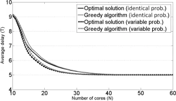
i ∈ [1, k], j ∈ [1, r] Pr(j ∈ Si) = q = 0.5. Fig. 4 presents the obtained average delay (in time slots) as a function of the number of cores.
We assume a first subcase in which all types haveidentical probabilities of 1k = 0.125. For a given set of types and a maximal value of N cores, we compare the average delay obtained by the (first) greedy algorithm with the minimal possible delay found while considering all possible solutions satisfying the constraint on the number of cores. Here, the total number of solutions for each input isG(k= 8) = 4140. Clearly, the minimal value of N that guarantees that all tasks can be satisfied is N = r = 10. In addition, the maximal observed total number of tasks in the k= 8 types is smaller than 60. Thus, we examine the values of N ∈ [10,60]. The results are presented in the first two upper curves in Fig. 4. For example, for large enough values of N, each type has its own pipeline and the average delay equals the average number of tasks per type, r·q= 10·0.5 = 5. In general, the average delay obtained by the greedy algorithm is relatively close to the optimal delay and it becomes even closer for larger N. For instance, for N = 16 the average greedy delay is 8.470, larger by 4.4% than the optimal delay of 8.110. This option suggests a reduction of (60−16)/60 = 73.3%in the number of cores with a cost of a delay larger by70% or 62.8%. For
N = 40 the delay of the greedy is 5.122 when the minimal possible average delay (5.112) is smaller by less than 0.2%. The average difference, for N ∈ [10,60], between the two delays is 0.103 time slots.
For the presented scheme of the selection of the tasks, we examine also a second subcase in which the types appear with
variable probabilities. We set the probabilities to be geometri-cally decreasing such that thek= 8probabilities of thektypes areα·2−1, α·2−2, α·2−3, α·2−4, α·2−5, α·2−6, α·2−7, α·2−8 forα= 256/255. These non-homogenous probabilities enable us to distinguish between the types to further improve the obtained average delay. For instance, we might prefer to have a dedicated pipeline for the most common type containing only cores for its required tasks. The observed delays, again by the greedy algorithm and the exhaustive search are illustrated in the two additional curves in Fig. 4. For instance, again for
[image:11.612.351.525.55.156.2]N = 16 the observed average delays are 7.310 and 7.090,
Fig. 4. Average delay (in time slots) as a function of the number of available cores (N) for the first experiment with synthetic data. Here, the probability for a packet type to require each task is 0.5. The two upper curves present the delay when thek= 8types appear with a uniform distribution. The two bottom curves examine the case where the types appear with geometrically-decreasing probabilities. The results are based on the average of103 experiments. The greedy algorithm performs relatively close to the optimal one.
Fig. 5. The average delay (in time slots) as a function of the number of available cores (N) for the second experiment with synthetic data. Here, the probability for a packet type to require each task is either 0.9 or 0.1, according to one of three predetermined distributions. The two upper curves present the delay when thek= 8types appear with a uniform distribution. The two bottom curves examine the case where the types appear with geometrically-decreasing probabilities. The results are based on the average of103experiments. Again, the greedy algorithm achieves close-to-optimal results.
respectively. Both delays are shorter by approximately a single time slot than the corresponding delays in the homogenous case. Here, the average difference between the average delay of the greedy algorithm and the minimal possible average delay is even shorter and equals0.061time slots.
We also want to check whether a possible dependency be-tween the different types can further improve the effectiveness of our approach. In a second experiment, the tasks required by the types are selected in a different manner. We first randomly produce three task distributions. Each distribution randomly defines for each of thertasks whether it will be required with a high probability of0.9or only with a smaller probability of0.1. For each task, both options are obtained with equal probabilities of 0.5. Next, each of the k = 8 types is assigned with a distribution and its tasks are randomly selected accordingly. In this experiment, the probability of a type to require a task is 0.5·0.9 + 0.5·0.1 = 0.5, as in the first experiment. The results are displayed in Fig. 5.
[image:11.612.351.528.248.350.2]TABLE I
SUMMARY OF THE SYNTHETIC EXPERIMENTS FOR THE AVERAGE DELAY FORN∈[10,60]
(A) Average value of the delay (in time slots) Experiment Identical Prob. Variable Prob.
Greedy Optimal Greedy Optimal (i) Independent 6.197 6.094 5.788 5.726
types
(ii) Distribution-based 5.652 5.603 5.515 5.469 types
(B) Delay forN= 16(in time slots)
Experiment Identical Prob. Variable Prob. Greedy Optimal Greedy Optimal (i) Independent 8.470 8.110 7.310 7.090
types
(ii) Distribution-based 6.802 6.649 6.401 6.223 types
Fig. 6. The worst-case delay (in time slots) as a function of the number of available cores (N) (with the same scale as in Fig. 4 and Fig. 5). The worst-case delay is independent of the probabilities of the different packet types and accordingly we do not distinguish between the two options of these probabilities. The two upper curves present the delay when thek= 8types are drawn independently (as in Fig. 4). The two bottom curves examine the case where the types are drawn based on one of three task distributions (as in Fig. 5). In all cases, the worst-case delay is not shorter (and in most cases longer) than the average delay in the corresponding experiment. In this experiment, the delays obtained by greedy algorithm are even closer to the optimal delays.
subcase, with identical probabilities for thektypes, illustrated in two upper curves, the average (over N ∈ [10,60]) of the optimal delay is 5.603 in comparison with a corresponding average delay of 6.094 in the first experiment. Likewise, for
N = 16 the greedy delay is 6.802 and the optimal delay is 6.649. In the second subcase, with non-homogenous probabili-ties, as shown in the two last curves, the average optimal delay is even shorter and equals 5.469. Here, forN = 16the delay of the greedy algorithm is 6.401 and of the optimal equals 6.223 time slots. The results, in both experiments, of the average delay (over N∈[10,60]) and the obtained delays for N= 16
are summarized in Table I.
We now examine the worst-case delay in the same synthetic simulations. We again compare the results of the relevant greedy algorithm with the optimal solution. Since the prob-abilities for the different packet types do not influence the worst-case delay, we do not distinguish between the two op-tions discussed above of identical or geometrically decreasing probabilities. However, the dependency between the sets of tasks (selected independently or according to one of three task distributions) is still important.
The results are based again on the average of 103
experi-TABLE II
SUMMARY OF THE SYNTHETIC EXPERIMENTS FOR THE WORST-CASE DELAY FORN∈[10,60]
(A) Average value of the delay (in time slots) Experiment Greedy Optimal (i) Independent types 7.838 7.820 (ii) Distribution-based types 7.162 7.158
(B) Delay forN= 16(in time slots) Experiment Greedy Optimal (i) Independent types 9.369 9.273 (ii) Distribution-based types 7.699 7.678
ments and are presented in Fig. 6. The two upper curves present the delay when the k= 8 types are drawn independently (as in Fig. 4). The two bottom curves examine the case where the types are drawn based on one of three task distributions (as in Fig. 5). For this metric of the worst-case delay, the results of the (second) greedy algorithm are even closer to the optimal solution. For the independent types, the average value of the optimal worst-case delay is 7.820 while the greedy algorithm obtains an average value of 7.838 (larger by only
0.23%). The obtained values of the worst-case delays are of course larger than the corresponding values of the average delays discussed earlier. When the sets of tasks are selected based on one of predetermined distributions, the delays are shorter and equals 7.158 and 7.162, respectively. Considering again the independent sets of tasks, the value of the optimal worst-case delay whenN = 16equals 9.273 time slots. When the number of cores is N = 60, the k = 8 pipelines can be served separately and the value of the worst-case delay equals the average value of the maximal number of tasks per type, 7.196. A short summary of the results is given also in Table II. As demonstrated in Example 3, there often exists a tradeoff between the two metrics of the average delay and the worst-case delay. We study this tradeoff by comparing both delays of the solutions for the two greedy algorithms. The first algorithm that tries to minimize the average delay, might achieve far-from-optimal worst-case delay while the second algorithm that optimizes the worst-case delay can result in a relatively high average delay. We examine this for the same instance from Fig. 4 (k = 8 types with r = 10 distinct tasks, each required with probability of 0.5 by each type, identical type probabilities, 103 experiments). The results are illustrated in Fig. 7 and Fig. 8.
Fig. 7(a) shows the result of the first algorithm for mini-mizing average delay and Fig. 7(b) the results of the second algorithm for minimizing worst-case delay. ForN ∈[10,60], in (a) the average value of the average delay is 6.197 and that of the worst-case delay is 8.05. In (b), the average value of the average delay is 6.709 and that of the worst-case delay is 7.811. As expected, they are much closer in (b) that optimizes the worst-case delay, which is always larger.
Number of cores (N)
10 20 30 40 50 60
Delay (time slots)
4 5 6 7 8 9 10
Worst-case delay (D) Average delay (T)
(a) Algorithm for minimizing theaveragedelay
Number of cores (N)
10 20 30 40 50 60
Delay (time slots)
4 5 6 7 8 9 10
Worst-case delay (D) Average delay (T)
[image:13.612.69.543.61.177.2](b) Algorithm for minimizing theworst-casedelay
Fig. 7. Algorithm comparison: The worst-case and average delay in the results of the two algorithms. In (a), the algorithm for minimizing average delay. In (b), the algorithm for minimizing worst-case delay. For both algorithms, minimizing one delay results in an increase for the other.
Number of cores (N)
10 20 30 40 50 60
Delay ratio
0.9 1 1.1 1.2 1.3 1.4 1.5
Average delay minimization Worst-case delay minimization
(a) Ratio of worst-case delay and average delay
Number of cores (N)
10 20 30 40 50 60
Increase
0.9 1 1.1 1.2 1.3 1.4 1.5
Average delay Worst-case delay
[image:13.612.68.543.226.341.2](b) Increase in each of the delays by minimizing the other
Fig. 8. Algorithm comparison: (a) presents the ratio of the worst-case delay and the average delay in both algorithms. The ratio is smaller when the worst-case delay is minimized. (b) illustrates the relative increase of each of the delays as a result of minimizing the other.
Number of cores (N)
10 50 100 150 200 250 300 350 400
Average delay (T)
0 10 20 40 60 80
r = 10 tasks r = 20 tasks r = 40 tasks r = 80 tasks
(a) Average-case delay vs. number of distinct tasks(r)
Number of cores (N)
10 20 40 60 80 100 120 140 160 180 200
Worst-case delay (D)
4 5 6 7 8 9 10
k = 4 types k = 8 types k = 16 types k = 32 types k = 64 types k = 128 types
(b) Worst-case delay vs. packet types number(k)
Fig. 9. Algorithm scalability: (a) presents the average delay as a function of the number of distinct tasks(r)(withk=8 packet types). (b) describes the worst-case delay as a function of the number of packet types number(k)(withr=10 distinct tasks). Results are calculated based on the corresponding greedy algorithms.
cores (where the solution is often composed of a single pipeline with all cores), for larger values of N ∈ [10,60] we can see different ratios in the two algorithms. In the first algorithm the ratio grows up to 1.443, while in the second the maximal value of the ratio is 1.239. Fig. 8(b) describes the increase in each of the delays achieved by running the other algorithm. The worst-case delay increases by up to 8.4% by using solutions for the first algorithm. For a large enough number of cores, the solution of the first algorithm serves each type separately and also often achieves an optimal worst-case delay that equals the largest demand in the input. For the average delay, the increase is larger and can equal up to 16.5%. This larger increase follows an inherent property of the algorithm for minimizing the worst-case delay that simplifies its input by colliding two types when
the required tasks of one is a subset of the demand of another. Thus a type can often be served unnecessarily by a longer pipeline. While this never influences the worst-case delay, it can increase the average delay. Accordingly, even for a large number of cores, we can see an increase in the average delay considering solutions of the second algorithm.
[image:13.612.68.545.390.509.2]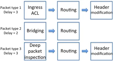
![Fig. 3.Three cases of the form of two consecutive (range) sets of tasksS Si = [Xi, Yi], Si+1 = [Xi+1, Yi+1] satisfying Xi < Xi+1](https://thumb-us.123doks.com/thumbv2/123dok_us/8350655.309621/9.612.57.566.54.144/fig-cases-form-consecutive-range-sets-taskss-satisfying.webp)