Unsupervised Learning
Unsupervised vs Supervised Learning:
• Most of this course focuses on supervised learningmethods such as regression and classification.
• In that setting we observe both a set of features
X1, X2, . . . , Xp for each object, as well as a response or
outcome variable Y. The goal is then to predictY using
X1, X2, . . . , Xp.
• Here we instead focus on unsupervised learning, we where observe only the features X1, X2, . . . , Xp. We are not
interested in prediction, because we do not have an associated response variable Y.
The Goals of Unsupervised Learning
• The goal is to discover interesting things about the
measurements: is there an informative way to visualize the data? Can we discover subgroups among the variables or among the observations?
• We discuss two methods:
• principal components analysis, a tool used for data visualization or data pre-processing before supervised techniques are applied, and
The Challenge of Unsupervised Learning
• Unsupervised learning is more subjective than supervised learning, as there is no simple goal for the analysis, such as prediction of a response.
• But techniques for unsupervised learning are of growing importance in a number of fields:
• subgroups of breast cancer patients grouped by their gene expression measurements,
• groups of shoppers characterized by their browsing and purchase histories,
• movies grouped by the ratings assigned by movie viewers.
Another advantage
• It is often easier to obtainunlabeled data — from a lab instrument or a computer — than labeled data, which can require human intervention.
Principal Components Analysis
• PCA produces a low-dimensional representation of a dataset. It finds a sequence of linear combinations of the variables that have maximal variance, and are mutually uncorrelated.
• Apart from producing derived variables for use in
supervised learning problems, PCA also serves as a tool for data visualization.
Principal Components Analysis: details
• The first principal componentof a set of featuresX1, X2, . . . , Xp is the normalized linear combination of the
features
Z1 =φ11X1+φ21X2+. . .+φp1Xp
that has the largest variance. By normalized, we mean that
Pp
j=1φ2j1= 1.
• We refer to the elementsφ11, . . . , φp1 as the loadings of the
first principal component; together, the loadings make up the principal component loading vector,
φ1 = (φ11φ21 . . . φp1)T.
PCA: example
10 20 30 40 50 60 70
0
5
10
15
20
25
30
35
Population
Ad Spending
The population size (pop) and ad spending (ad) for 100 different
cities are shown as purple circles. The green solid line indicates the first principal component direction, and the blue dashed line indicates the second principal component direction.
Computation of Principal Components
• Suppose we have a n×pdata set X. Since we are only interested in variance, we assume that each of the variables inX has been centered to have mean zero (that is, the column means ofX are zero).
• We then look for the linear combination of the sample feature values of the form
zi1 =φ11xi1+φ21xi2+. . .+φp1xip (1)
fori= 1, . . . , n that has largest sample variance, subject to
the constraint that Pp
j=1φ2j1 = 1.
• Since each of the xij has mean zero, then so does zi1 (for
any values of φj1). Hence the sample variance of the zi1
can be written as 1nPn
Computation: continued
• Plugging in (1) the first principal component loading vector solves the optimization problem
maximize
φ11,...,φp1
1
n n
X
i=1
p
X
j=1
φj1xij
2
subject to
p
X
j=1
φ2j1= 1.
• This problem can be solved via a singular-value
decomposition of the matrix X, a standard technique in linear algebra.
• We refer toZ1 as the first principal component, with
realized values z11, . . . , zn1
Geometry of PCA
• The loading vectorφ1 with elementsφ11, φ21, . . . , φp1
defines a direction in feature space along which the data vary the most.
• If we project the ndata points x1, . . . , xn onto this
Further principal components
• The second principal component is the linear combination
of X1, . . . , Xp that has maximal variance among all linear
combinations that are uncorrelatedwithZ1.
• The second principal component scores z12, z22, . . . , zn2
take the form
zi2 =φ12xi1+φ22xi2+. . .+φp2xip,
where φ2 is the second principal component loading vector,
with elementsφ12, φ22, . . . , φp2.
Further principal components: continued
• It turns out that constrainingZ2 to be uncorrelated with Z1 is equivalent to constraining the directionφ2 to be
orthogonal (perpendicular) to the direction φ1. And so on.
• The principal component directionsφ1,φ2,φ3, . . . are the
Illustration
• USAarrests data: For each of the fifty states in the United
States, the data set contains the number of arrests per 100,000 residents for each of three crimes: Assault,Murder,
and Rape. We also record UrbanPop (the percent of the
population in each state living in urban areas).
• The principal component score vectors have length n= 50, and the principal component loading vectors have length
p= 4.
• PCA was performed after standardizing each variable to have mean zero and standard deviation one.
USAarrests data: PCA plot
−3 −2 −1 0 1 2 3
−3 −2 −1 0 1 2 3
First Principal Component
Second Pr incipal Component Alabama Alaska Arizona Arkansas California Colorado Connecticut Delaware Florida Georgia Hawaii Idaho Illinois Indiana Iowa Kansas Kentucky Louisiana Maine Maryland Massachusetts Michigan Minnesota Mississippi Missouri Montana Nebraska Nevada New Hampshire New Jersey New Mexico New York North Carolina North Dakota Ohio Oklahoma Oregon Pennsylvania Rhode Island South Carolina
South Dakota Tennessee
Texas Utah Vermont Virginia Washington West Virginia Wisconsin Wyoming
−0.5 0.0 0.5
Figure details
The first two principal components for the USArrests data.
• The blue state names represent the scores for the first two principal components.
• The orange arrows indicate the first two principal component loading vectors (with axes on the top and right). For example, the loading for Rape on the first
component is 0.54, and its loading on the second principal component 0.17 [the wordRapeis centered at the point
(0.54,0.17)].
• This figure is known as a biplot, because it displays both the principal component scores and the principal
component loadings.
PCA loadings
PC1 PC2
Another Interpretation of Principal Components
First principal component
Second principal component
−1.0 −0.5 0.0 0.5 1.0
−1.0 −0.5 0.0 0.5 1.0 • • • • • • • • • • • • • • • • • • • • • • • • • • • • • • • • • • • • • • • • • • • • • • • • • • • • • • • • • • • • • • • • • • • • • • • • • • • • • • • • • • • • • • • • • •
PCA find the hyperplane closest to the observations
• The first principal component loading vector has a very special property: it defines the line in p-dimensional space that is closest to thenobservations (using average squared Euclidean distance as a measure of closeness)
• The notion of principal components as the dimensions that are closest to the nobservations extends beyond just the first principal component.
Scaling of the variables matters
• If the variables are in different units, scaling each to have standard deviation equal to one is recommended.
• If they are in the same units, you might or might not scale the variables.
−3 −2 −1 0 1 2 3
−3 −2 −1 0 1 2 3
First Principal Component
Second Pr incipal Component * * * * * * * * * * * * * * * * * * * * * * * * * * * * * * * * * * * ** * * * * * * * * * * * * *
−0.5 0.0 0.5
−0.5 0.0 0.5 Murder Assault UrbanPop Rape Scaled
−100 −50 0 50 100 150
−100 −50 0 50 100 150
First Principal Component
Second Pr incipal Component * * * * * * * * * * * * * * * * ** * * * * * * * * * * * * * * * * * * * * * * * * * * * * * * * *
−0.5 0.0 0.5 1.0
−0.5 0.0 0.5 1.0 Murder Assault UrbanPop Rape Unscaled
Proportion Variance Explained
• To understand the strength of each component, we are interested in knowing the proportion of variance explained (PVE) by each one.
• The total variance present in a data set (assuming that the variables have been centered to have mean zero) is defined as
p
X
j=1
Var(Xj) = p X j=1 1 n n X i=1
x2ij,
and the variance explained by themth principal component is
Var(Zm) =
1
n n
X
i=1
z2im.
• It can be shown thatPp
j=1Var(Xj) =PMm=1Var(Zm),
Proportion Variance Explained: continued
• Therefore, the PVE of the mth principal component isgiven by the positive quantity between 0 and 1
Pn
i=1z2im
Pp
j=1
Pn
i=1x2ij
.
• The PVEs sum to one. We sometimes display the cumulative PVEs.
1.0 1.5 2.0 2.5 3.0 3.5 4.0
0.0 0.2 0.4 0.6 0.8 1.0 Principal Component Prop . V ar iance Explained
1.0 1.5 2.0 2.5 3.0 3.5 4.0
0.0 0.2 0.4 0.6 0.8 1.0 Principal Component Cum ulativ e Prop . V ar iance Explained
How many principal components should we use?
If we use principal components as a summary of our data, how many components are sufficient?
• No simple answer to this question, as cross-validation is not available for this purpose.
• Why not?
• When could we use cross-validation to select the number of components?
• the “scree plot” on the previous slide can be used as a guide: we look for an “elbow”.
How many principal components should we use?
If we use principal components as a summary of our data, how many components are sufficient?
• No simple answer to this question, as cross-validation is not available for this purpose.
• Why not?
• When could we use cross-validation to select the number of components?
Clustering
• Clustering refers to a very broad set of techniques for finding subgroups, orclusters, in a data set.
• We seek a partition of the data into distinct groups so that the observations within each group are quite similar to each other,
• It make this concrete, we must define what it means for two or more observations to be similarordifferent.
• Indeed, this is often a domain-specific consideration that must be made based on knowledge of the data being studied.
PCA vs Clustering
• PCA looks for a low-dimensional representation of the observations that explains a good fraction of the variance.
Clustering for Market Segmentation
• Suppose we have access to a large number of measurements (e.g. median household income, occupation, distance from nearest urban area, and so forth) for a large number of people.
• Our goal is to perform market segmentationby identifying subgroups of people who might be more receptive to a particular form of advertising, or more likely to purchase a particular product.
• The task of performing market segmentation amounts to clustering the people in the data set.
Two clustering methods
• In K-means clustering, we seek to partition the observations into a pre-specified number of clusters.
• In hierarchical clustering, we do not know in advance how many clusters we want; in fact, we end up with a tree-like visual representation of the observations, called a
K
-means clustering
K=2 K=3 K=4
A simulated data set with 150 observations in 2-dimensional space. Panels show the results of applyingK-means clustering with different values ofK, the number of clusters. The color of each observation indicates the cluster to which it was assigned using theK-means clustering algorithm. Note that there is no ordering of the clusters, so the cluster coloring is arbitrary. These cluster labels were not used in clustering; instead, they are the outputs of the clustering procedure.
Details of
K
-means clustering
LetC1, . . . , CK denote sets containing the indices of the
observations in each cluster. These sets satisfy two properties:
1. C1∪C2∪. . .∪CK ={1, . . . , n}. In other words, each
observation belongs to at least one of the K clusters.
2. Ck∩Ck0 =∅ for allk6=k0. In other words, the clusters are
non-overlapping: no observation belongs to more than one cluster.
For instance, if theith observation is in the kth cluster, then
Details of
K
-means clustering: continued
• The idea behind K-means clustering is that agoodclustering is one for which thewithin-cluster variation is as small as possible.
• The within-cluster variation for clusterCk is a measure
WCV(Ck) of the amount by which the observations within
a cluster differ from each other.
• Hence we want to solve the problem
minimize
C1,...,CK
( K
X
k=1
WCV(Ck)
)
. (2)
• In words, this formula says that we want to partition the observations into K clusters such that the total
within-cluster variation, summed over all K clusters, is as small as possible.
How to define within-cluster variation?
• Typically we use Euclidean distance
WCV(Ck) =
1
|Ck|
X
i,i0∈C k
p
X
j=1
(xij−xi0j)2, (3)
where |Ck|denotes the number of observations in the kth
cluster.
• Combining (2) and (3) gives the optimization problem that defines K-means clustering,
minimize
C1,...,CK
K X k=1 1
|Ck|
X
i,i0∈C k
p
X
j=1
(xij −xi0j)2
K
-Means Clustering Algorithm
1. Randomly assign a number, from 1 to K, to each of the observations. These serve as initial cluster assignments for the observations.
2. Iterate until the cluster assignments stop changing:
2.1 For each of theK clusters, compute the clustercentroid. Thekth cluster centroid is the vector of thepfeature means for the observations in thekth cluster.
2.2 Assign each observation to the cluster whose centroid is closest (whereclosest is defined using Euclidean distance).
Properties of the Algorithm
• This algorithm is guaranteed to decrease the value of the objective (4) at each step. Why?
Note that
1
|Ck|
X
i,i0∈C k
p
X
j=1
(xij −xi0j)2= 2
X
i∈Ck
p
X
j=1
(xij −x¯kj)2,
where ¯xkj = |C1 k|
P
i∈Ckxij is the mean for featurej in
cluster Ck.
• however it is not guaranteed to give the global minimum.
Properties of the Algorithm
• This algorithm is guaranteed to decrease the value of the objective (4) at each step. Why? Note that
1
|Ck|
X
i,i0∈C k
p
X
j=1
(xij −xi0j)2= 2
X
i∈Ck
p
X
j=1
(xij −x¯kj)2,
where ¯xkj = |C1k|
P
i∈Ckxij is the mean for featurej in
cluster Ck.
• however it is not guaranteed to give the global minimum.
Why not?
Example
Data Step 1 Iteration 1, Step 2a
Details of Previous Figure
The progress of the K-means algorithm withK=3.
• Top left: The observations are shown.
• Top center: In Step 1 of the algorithm, each observation is randomly assigned to a cluster.
• Top right: In Step 2(a), the cluster centroids are computed. These are shown as large colored disks. Initially the
centroids are almost completely overlapping because the initial cluster assignments were chosen at random.
• Bottom left: In Step 2(b), each observation is assigned to the nearest centroid.
• Bottom center: Step 2(a) is once again performed, leading to new cluster centroids.
• Bottom right: The results obtained after 10 iterations.
Example: different starting values
320.9 235.8 235.8
Details of Previous Figure
K-means clustering performed six times on the data from previous figure withK = 3, each time with a different random assignment of the observations in Step 1 of theK-means algorithm.
Above each plot is the value of the objective (4).
Three different local optima were obtained, one of which resulted in a smaller value of the objective and provides better separation between the clusters.
Those labeled in red all achieved the same best solution, with an objective value of 235.8
Hierarchical Clustering
• K-means clustering requires us to pre-specify the number of clusters K. This can be a disadvantage (later we discuss strategies for choosing K)
• Hierarchical clustering is an alternative approach which does not require that we commit to a particular choice of
K.
• In this section, we describe bottom-uporagglomerative
Hierarchical Clustering: the idea
Builds a hierarchy in a “bottom-up” fashion...
A B
C
D
E
Hierarchical Clustering: the idea
Builds a hierarchy in a “bottom-up” fashion...
A B
C
D
Hierarchical Clustering: the idea
Builds a hierarchy in a “bottom-up” fashion...
A B
C
D
E
Hierarchical Clustering: the idea
Builds a hierarchy in a “bottom-up” fashion...
A B
C
D
Hierarchical Clustering: the idea
Builds a hierarchy in a “bottom-up” fashion...
A B
C
D
E
Hierarchical Clustering Algorithm
The approach in words:
• Start with each point in its own cluster.
• Identify the closest two clusters and merge them.
• Repeat.
• Ends when all points are in a single cluster.
A B
C
D E
0
1
2
3
4
Dendrogram
Hierarchical Clustering Algorithm
The approach in words:
• Start with each point in its own cluster.
• Identify theclosesttwo clusters and merge them.
• Repeat.
• Ends when all points are in a single cluster.
A B
C
D E
0
1
2
3
4
Dendrogram
D E B A C
An Example
−6 −4 −2 0 2
−2
0
2
4
X1
X2
Application of hierarchical clustering
0
2
4
6
8
10
0
2
4
6
8
10
0
2
4
6
8
10
Details of previous figure
• Left: Dendrogram obtained from hierarchically clustering the data from previous slide, with complete linkage and Euclidean distance.
• Center: The dendrogram from the left-hand panel, cut at a height of 9 (indicated by the dashed line). This cut results in two distinct clusters, shown in different colors.
Another Example
3 4 1 6 9 2 8 5 7 0.0 0.5 1.0 1.5 2.0 2.5 3.0 1 2 3 4 5 6 7 8 9−1.5 −1.0 −0.5 0.0 0.5 1.0
−1.5 −1.0 −0.5 0.0 0.5 X1 X 2
• An illustration of how to properly interpret a dendrogram with nine observations in two-dimensional space. The raw data on the right was used to generate the dendrogram on the left.
• Observations 5 and 7 are quite similar to each other, as are observations 1 and 6.
• However, observation 9 is no more similar toobservation 2 than it is to observations 8,5,and 7, even though observations 9 and 2 are close together in terms of horizontal distance.
• This is because observations 2,8,5,and 7 all fuse with observation 9 at the same height, approximately 1.8.
Merges in previous example
1 2 3 4 5 6 7 8 9−1.5 −1.0 −0.5 0.0 0.5 1.0
−1.5 −1.0 −0.5 0.0 0.5 1 2 3 4 5 6 7 8 9
−1.5 −1.0 −0.5 0.0 0.5 1.0
−1.5 −1.0 −0.5 0.0 0.5 1 2 3 4 5 6 7 8 9
−1.5 −1.0 −0.5 0.0 0.5 1.0
−1.5 −1.0 −0.5 0.0 0.5 1 2 3 4 5 6 7 8 9
−1.5 −1.0 −0.5 0.0 0.5 1.0
Types of Linkage
Linkage Description
Complete
Maximal inter-cluster dissimilarity. Compute all pairwise dissimilarities between the observations in cluster A and the observations in cluster B, and record the largest of these dissimilarities.
Single
Minimal inter-cluster dissimilarity. Compute all pairwise dissimilarities between the observations in cluster A and the observations in cluster B, and record thesmallestof these dissimilarities.
Average
Mean inter-cluster dissimilarity. Compute all pairwise dissimilarities between the observations in cluster A and the observations in cluster B, and record theaverage of these dissimilarities.
Centroid
Dissimilarity between the centroid for cluster A (a mean vector of lengthp) and the centroid for cluster B. Cen-troid linkage can result in undesirableinversions.
Choice of Dissimilarity Measure
• So far have used Euclidean distance.• An alternative iscorrelation-based distance which considers two observations to be similar if their features are highly correlated.
• This is an unusual use of correlation, which is normally computed between variables; here it is computed between the observation profiles for each pair of observations.
5 10 15 20
0
5
10
15
20 Observation 1
Observation 2 Observation 3
1
2
Scaling of the variables matters
Socks Computers
0
2
4
6
8
10
Socks Computers
0.0
0.2
0.4
0.6
0.8
1.0
1.2
Socks Computers
0
500
1000
1500
Practical issues
• Should the observations or features first be standardized in some way? For instance, maybe the variables should be centered to have mean zero and scaled to have standard deviation one.
• In the case of hierarchical clustering,
• What dissimilarity measure should be used?
• What type of linkage should be used?
Example: breast cancer microarray study
• “Repeated observation of breast tumor subtypes in
independent gene expression data sets;” Sorlie at el, PNAS 2003
• Average linkage, correlation metric
• Clustered samples using 500 intrinsic genes: each woman was measured before and after chemotherapy. Intrinsic genes have smallest within/between variation.
Westet al.data sets (Table 4). We note that prediction accuracies reported above are somewhat optimistic, as some of the genes used as predictors were used to define the test set groups in the first place.
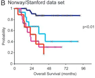
Tumor Subtypes Are Associated with Significant Difference in Clinical Outcome.In our previous work, the expression-based tumor sub-types were associated with a significant difference in overall survival as well as disease-free survival for the patients suffering from locally advanced breast cancer and belonging to the same treatment protocol (6). To investigate whether these subtypes were also associated with a significant difference in outcome in other patient cohorts, we performed a univariate Kaplan–Meier analysis with time to development of distant metastasis as a variable in the data
set comprising the 97 sporadic tumors taken from van’t Veeret al.
As shown in Fig. 5, the probability of remaining disease-free was significantly different between the subtypes; patients with luminal A type tumors lived considerably longer before they developed
metastatic disease, whereas the basal and ERBB2⫹groups showed
much shorter disease-free time intervals. Although the method-ological differences prevent a definitive interpretation, it is notable that the order of severity of clinical outcome associated with the several subtypes is similar in the two dissimilar cohorts. We could
not carry out a similar analysis in the Westet al.data because the
necessary follow-up data were not provided.
Discussion
Breast Tumor Subtypes Represent Distinct Biological Entities.Gene expression studies have made it clear that there is considerable diversity among breast tumors, both biologically and clinically (5, 6,
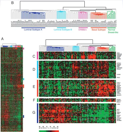
Fig. 1. Hierarchical clustering of 115 tumor tissues and 7 nonmalignant tissues using the ‘‘intrinsic’’ gene set. (A) A scaled-down representation of the entire cluster
of 534 genes and 122 tissue samples based on similarities in gene expression. (B) Experimental dendrogram showing the clustering of the tumors into five subgroups. Branches corresponding to tumors with low correlation to any subtype are shown in gray. (C) Gene cluster showing theERBB2oncogene and other coexpressed genes. (D) Gene cluster associated with luminal subtype B. (E) Gene cluster associated with the basal subtype. (F) A gene cluster relevant for the normal breast-like group. (G) Cluster of genes including the estrogen receptor (ESR1) highly expressed in luminal subtype A tumors. Scale bar represents fold change for any given gene relative to the median level of expression across all samples. (See also Fig. 6.)
Another expectation from the concept that the tumor subtypes represent different biological entities is that genetic predispositions to breast cancer might give rise preferentially to certain subtypes. This expectation is amply fulfilled by our finding in the data of van’t
Veeret al., which shows that the women carryingBRCA1-mutated
alleles all had tumors with the basal-like gene expression pattern.
Tumor Subtypes and Clinical Outcome.Consistent with the results
previously found in our data (6), we also found differences in clinical outcome associated with the different tumor subtypes in the data set produced by van’t Veeret al. The outcomes, as measured here in time to development of distant metastasis, were strikingly similar to what we found previously: worst for basal (and ERBB2⫹), best for luminal A, and intermediate for luminal B subtypes. Recently, two reports corroborating the poor outcome of the basal subtype solely based on immunohistochemistry with antibodies against keratins 5 and 17 and Skp2, strongly supports our results (24, 25). The finding that our gene cluster profile was of similar prognostic importance in the van’t Veeret al.cohort as among our patients is remarkable, taking into account differences regarding disease stage (locally advanced versus stage I primaries) and patient age, but in particular, the fact that the Norwegian patients had presurgical chemotherapy and all patients expressing ESR1received adjuvant endocrine treatment, whereas the patients from van’t Veer et al. in general did not receive any systemic adjuvant treatment.
The observation thatBRCA1mutations are strongly associated with a basal tumor phenotype indicates a particularly poor prog-nosis for these patients. BRCA1-associated breast cancers are usually highly proliferative and TP53-mutated, and usually lack expression of ESR1 and ERBB2 (20, 26). Status of BRCA1 in familial cancers has failed to be an independent prognostic factor in several studies (reviewed in ref. 27), and is complicated by confounding factors such as frequent screening and early diagnosis.
Molecular Marker Identification.In a mixture of biologically distinct
subtypes, it may well be that individual markers derived by super-vised analysis will under-perform what is possible if tumor subtypes were separated before searching, in a supervised fashion, for prognostic indicators. Indeed, when we tested the prognostic impact of the 231 markers published by van’t Veeret al.on the Norwegian cohort, we found that they performed less well (47%) in predicting recurrences within 5 years (seeMaterials and Methods). This may in part be due to differences in the patient cohorts and treatments as discussed above.
Both van’t Veeret al.and Westet al.showed the ability of gene
Fig. 4. Hierarchical clustering of gene expression
data from Westet al. (A) Scaled-down representation of the full cluster of 242 intrinsic genes across 49 breast tumors. (B) Dendrogram displaying the relative orga-nization of the tumor samples. Branches are colored according to which subtype the corresponding tumor showed the strongest correlation with. Gray branches indicate tumors with low correlation (⬍0.1) to any specific subtype. (C) Luminal epithelial兾estrogen recep-tor gene cluster. (D) Basal gene cluster. (E) ERBB2⫹ gene cluster. (See also Fig. 9, which is published as supporting information on the PNAS web site.)
Fig. 5. Kaplan–Meier analysis of disease outcome in two patient cohorts. (A)
Time to development of distant metastasis in the 97 sporadic cases from van’t
Veeret al. Patients were stratified according to the subtypes as shown in Fig. 2B.
(B) Overall survival for 72 patients with locally advanced breast cancer in the Norway cohort. The normal-like tumor subgroups were omitted from both data sets in this analysis.
Conclusions
• Unsupervised learning is important for understanding the variation and grouping structure of a set of unlabeled data, and can be a useful pre-processor for supervised learning
• It is intrinsically more difficult than supervised learning
because there is no gold standard (like an outcome variable) and no single objective (like test set accuracy)
• It is an active field of research, with many recently developed tools such as self-organizing maps,independent components analysisand spectral clustering.