R E S E A R C H A R T I C L E
Open Access
Optimizing cost-efficiency in mean exposure
assessment - cost functions reconsidered
Svend Erik Mathiassen
1*and Kristian Bolin
2Abstract
Background:Reliable exposure data is a vital concern in medical epidemiology and intervention studies. The present study addresses the needs of the medical researcher to spend monetary resources devoted to exposure assessment with an optimal cost-efficiency, i.e. obtain the best possible statistical performance at a specified budget. A few previous studies have suggested mathematical optimization procedures based on very simple cost models; this study extends the methodology to cover even non-linear cost scenarios.
Methods:Statistical performance, i.e. efficiency, was assessed in terms of the precision of an exposure mean value, as determined in a hierarchical, nested measurement model with three stages. Total costs were assessed using a corresponding three-stage cost model, allowing costs at each stage to vary non-linearly with the number of measurements according to a power function. Using these models, procedures for identifying the optimally cost-efficient allocation of measurements under a constrained budget were developed, and applied on 225 scenarios combining different sizes of unit costs, cost function exponents, and exposure variance components.
Results:Explicit mathematical rules for identifying optimal allocation could be developed when cost functions were linear, while non-linear cost functions implied that parts of or the entire optimization procedure had to be carried out using numerical methods.
For many of the 225 scenarios, the optimal strategy consisted in measuring on only one occasion from each of as many subjects as allowed by the budget. Significant deviations from this principle occurred if costs for recruiting subjects were large compared to costs for setting up measurement occasions, and, at the same time, the between-subjects to within-subject variance ratio was small. In these cases, non-linearities had a profound influence on the optimal allocation and on the eventual size of the exposure data set.
Conclusions:The analysis procedures developed in the present study can be used for informed design of exposure assessment strategies, provided that data are available on exposure variability and the costs of collecting and processing data. The present shortage of empirical evidence on costs and appropriate cost functions however impedes general conclusions on optimal exposure measurement strategies in different epidemiologic scenarios.
Background
Reliable exposure assessment is a vital concern in medi-cal epidemiology and intervention research. In occupa-tional as well as public health studies, exposure is often monitored using equipment that allows data to be col-lected at a high resolution for long periods and on repeated occasions (e.g. [1-4]). A considerable emphasis has been put on developing and applying methods for analyzing sources of exposure variability in such data, in
terms of so-called variance components [5-8]. As an example, variance components pertaining to, e.g. com-panies, occupations, subjects, days within subjects, and exposure samples within days have been determined for a large number of airborne, dermal, and biomechanical exposures in working life (e.g. [2,3,9-15]). These variance components have been utilized as a remedy for identify-ing targets for surveillance, intervention and prevention [6,16,17], as well as for designing effective exposure assessment strategies producing information at a desired level of precision. While an extensive literature deals with the consequences of random exposure variability to bias and precision in exposure-outcome relationships * Correspondence: [email protected]
1
Centre for Musculoskeletal Research, Department of Occupational and Public Health Sciences, University of Gävle, Sweden
Full list of author information is available at the end of the article
[18-22], some attention has also been paid to the use of variance components for estimating sampling needs in studies examining compliance with exposure limits [6], and in studies comparing groups [12] or conditions [13] as in an intervention scenario. In the latter case, the requirement for reliable exposure data can be expressed as a need to obtain estimates of the mean exposure of individuals or groups with a sufficient precision to arrive at a confidence interval of acceptable size, or secure an acceptable statistical power in a specified hypothesis test. Generalized formulae are available for estimating statistical efficiency, i.e. the relationship between the precision of a mean exposure estimate, on the one hand, and, on the other, the size of relevant variance compo-nents, and the number of measurements at the corre-sponding sampling stages [23,24]. The most frequently applied measurement model is hierarchical and random with two or three nested stages, for instance subjects and days within subjects [2,25,26]; subjects, days within subjects and samples within days [12,27]; or groups, subjects within groups, and days within subjects [28]. A few attempts have been made to apply more compli-cated models, e.g. including crossed (non-nested) com-ponents related to the distribution of measurement days among subjects [29] or associated with methodological variance [11]. Also, mixed models including fixed deter-minants of exposure in addition to random effects are in increasing use [13,30-33].
Some studies have been devoted particularly to under-standing the effects on the precision of an estimated group mean exposure of allocating measurement efforts in different ways between and within subjects [12], between occupational recordings and data processing [11], or across time within a measurement day [34,35]. This had led to a number of principles for statistically efficient exposure assessment, i.e. measurement strate-gies that perform well at a specified investment of mea-surement resources, or, equivalently, yield a specified performance with comparatively small measurement efforts [12,34]. As one trivial conclusion, more data gen-erally leads to better statistical performance, and furthermore, efficiency increases if measurements are allocated to higher sampling stages in the hierarchical model [23].
At the same time, more measurements inevitably imply larger monetary costs. While budget constraints are the pragmatic reality in most exposure assessments, surprisingly few studies have addressed the issue of how to design a measurement strategy so as to give the best possible statistical efficiency at the availablemonetary resources [36]. This endeavor is not equivalent to addressing statistical efficiency per se, as introduced above, since measurements at different stages may entail different costs. For instance, increasing the number of
groups may be considerably more expensive than col-lecting data from more subjects in an existing group; and the process of identifying and approaching a new subject may be more expensive than achieving more measurements from a subject already in the sample population. Also, different measurement instruments yielding the same exposure variables may imply different costs, in particular if the risk of measurement failures is acknowledged [37]. Of the limited literature devoted to efficiencyandcost in data collection, some studies com-pare a selection of measurement strategies in order to identify the one superior in cost-efficiency [38-41]. A few studies take on the more challenging task of deter-mining theoptimally cost-efficient strategy at a certain budget, on the basis of specified costs for collecting data at different stages, and specified sizes of the correspond-ing variance components. The general significance of examining cost-efficiency in data collection is illustrated by previous studies appearing in a variety of research areas, including occupational hygiene [38], environmen-tal medicine [39,42,43], clinical chemistry [44], and nutrition [45].
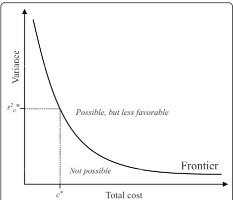
Basically, optimization in the case of exposure assess-ment strives to identify data collection strategies at the frontier of possible relationships between cost and sta-tistical efficiency (figure 1).
ance
Va
ri
a
Possible, but less favorable s2
ȝ*
Frontier
N t iblTotal cost
c*
Not possible
Figure 1The notion of optimal cost-efficiency. The horizontal axis illustrates the total cost associated with an exposure
Previous optimization studies have addressed hierarch-ical models with two [45-47] or three [43,44,47] stages, as well as the optimal allocation of measurements between two alternative yet correlated instruments for data collection [42,48,49]. All these studies have, how-ever, assumed that the price of one measurement unit at each stage is constant, implying that costs increase in a linear fashion at that stage, proportionally to the num-ber of samples. Only in an appendix of the paper by Duan and Mage [42], an empirical example appears of the quite likely case that costs may vary with the num-ber of measurements; for instance that subjects recruited late in a study may require more time for being per-suaded, and thus entail larger labor costs, than subjects signing up immediately. Also, in his textbook on sam-pling strategies, Cochran [47] reports some non-linear cost functions in other areas of data collection, and additional examples appear in Groves [50]. In addition, the cited cost-efficiency studies do not, in general, con-sider whether the identified optimal strategies are feasi-ble under the constraints dictated by a specified, yet limited budget.
Thus, the present paper is devoted to deriving meth-ods for optimizing exposure assessment strategies, in terms of offering the best possible trade-off between total costs and statistical efficiency. In contrast to pre-vious literature, this study explores optimal cost-effi-ciency even when cost functions are not linear and budget constraints apply, and the study also identifies alternative optimization procedures in those cases where analytical closed-form solutions cannot be developed.
First, the paper presents a general theoretical model of cost and efficiency when assessing exposure mean values in occupational groups, including some theoretical results based on that model. Then, the general model is simplified, and procedures are derived for identifying optimally cost-efficient exposure assessment strategies, depending on the shapes of cost functions. These results are illustrated by numerical examples. A general discus-sion on the representativeness and sensitivity of the sug-gested optimization procedures concludes the paper.
Methods
A framework for cost-efficient exposure assessment Exploring cost-efficiency at an ordinal level only requires a specification of the properties of the mathe-matical function associating each exposure assessment strategy with its stated statistical objective. If, however, the goal of the cost-efficiency analysis is to compare or optimize strategies in explicit, quantitative terms, speci-fic functional forms need be identified that parameterize objectives and costs. This is a necessary requirement when aiming at the (occasionally more than one) strat-egy that maximizes efficiency among the large selection
of possible assessment strategies entailing a particular cost.
Thus, three major issues must be considered as part of a quantitative analysis of cost-efficient resource con-sumption: (1) why resources are used, i.e. theobjective of collecting data, (2) how much resources are required to fulfil the objective, expressed in terms of unit-costs, and (3) whether the intended strategy for resource con-sumption is feasible. When examining cost-efficient assessments of group mean exposure we thus need to know (1) the relationship between the group mean and the assessment strategy, as reflected by what is usually referred to as the objective function, (2) the amount of monetary resources required to realise a particular assessment strategy, expressed by the cost function, and (3) the amount of monetary resources at our disposal, as reflected by thebudget constraint.
The objective function - precision of the mean
For a hierarchical three-stage balanced data set (sub-jects, occasions within subject, samples within occasion), the group mean exposure, μ, can be estimated using a “mean of means” approach [23] as:
μ= 1
ns
i (1
nd
j(i) (1
nq
k(ij)
xk(ij)))
Wherexk(ij)is an individual exposure sample, collected from subject ion occasion j;nsis the number of
sub-jects included in the data set; nd is the number of
dis-tinct measurement occasions, for instance days, per subject; andnqis the number of samples, or quanta, per
measurement occasion. Accordingly, averaging is made across quanta within each occasion, then across occa-sions within each subject, and finally across subjects.
A general formula for determining the variance of this group mean exposure estimate, s2μ, has been proposed and applied by several authors [12,23,44,47]. This objec-tive function takes the form:
s2μ(ns,nd,nq) =
s2BS+s 2
BD
nd + s
2
WD
nd·nq
ns (1)
The cost function
While all cost functions suggested in the literature have been linear, the cost associated with collectingnqquanta
on each of ndoccasions for each of ns subjects can be
assessed even in a non-linear case, provided that infor-mation is available on the“capability”to recruit subjects, that is, the amount of resources needed for recruiting any specific number of subjects, and the equivalent cap-abilities for setting up measurement occasions within each subject and collecting quanta within each occasion. Assume first that these three capabilities are all homo-geneous of degreek, in the sense that if all resources are multiplied by a certain factor, x (x > 1), output will increase by xk. This is a common assumption in eco-nomics addressing non-linear production capabilities. For example, ifk= 1 and resources allocated to the pro-cess of recruiting subjects are doubled, then the number of subjects recruited will also double; this is simple pro-portional linearity. In the case of k = 0.5, doubled recruitment resources would lead to an increase in the number of recruited subjects by a factor 21/2=√2.
Assume further that the resources needed for setting up nd measurement occasions, each containing nqquanta,
do not depend on the subject from whom data are col-lected, and the resources needed to collectnqquanta on
a particular measurement occasion for a particular sub-ject are independent of occasion and subsub-ject.
The first of these two assumed capability properties allows cost functions for recruiting subjects, cs, setting
up measurement occasions within each subject,cd, and
collecting measurement quanta within each occasion,cq,
to be expressed as:cs(ns) =πs·nαs; cd(nd) =πd·nβd; and
cq(nq) =πq·nγq,
where the π-values are the costs for obtaining one measurement unit at each stage of data collection, so-called unit costs, anda,bandgare parameters, all lar-ger than 0, describing the shape of a power relationship between the number of measurement units and costs.
The relationship between the value(s) of πand the exponents a, b and g can be illustrated by examining the cost functions. If, for instance, a = 1, the cost of recruiting ns subjects is cs(ns) = πs ⋅ns, i.e. the cost
increases in direct proportion to the number of subjects. In this case,πsis the one-unit cost (cs(1) =πs), as well
as the marginal cost of recruiting any additional subject (∂cs/∂ns=πs). Ifa≠1,πsis still the one-unit cost, but the marginal cost is now∂cs
∂ns =πs·α·nαs−1. Thus, if a> 1, the marginal cost of including an additional sub-ject increases with the number of subsub-jects, while it decreases when 0 <a< 1.
The second capability property assumed above implies that the total cost of collecting a data set including ns
subjects each observed forndoccasions, each containing
nq quanta can be stated ascs(ns) +nscd(nd) +nsndcq
(nq), which equals:
c(ns,nd,nq) =πs·nαs +πd·ns·nβd +πq·ns·nd·nγq (2)
This cost function presents a generalisation of pre-viously suggested linear cost functions [43,44,46] by per-mitting both linear and non-linear relationships between the sample size at different stages of data collection and the cost of obtaining data. With (a,b,g) = (1,1,1), equa-tion (2) takes the customary linear form used in pre-vious studies. Notably, equation (2) only expresses the variable costs associated with measurement; possible fixed costs, which do not depend on the number of samples, need to be added to give the total cost of col-lecting the data set, but will not affect the optimization procedures developed below [41,43].
The general optimization problem
If a data collection is allowed to consume a total budget R(after possible reduction by fixed costs), combinations of ns,nd andnq that optimize the output, i.e. minimize
the resulting variance of the estimated mean exposure, can be retrieved by solving the following optimization problem:
Minimize s2μ(ns,nd,nq) =
s2BS+s 2
BD
nd + s
2
WD
nd·nq
ns
with respect tons, nd, nq; subject to the constraint:
c(ns,nd,nq) =πs·nαs +πd·ns·nβd +πq·ns·nd·nγq ≤R,
ns≥1;nd≥1;nq≥1.
Due to the non-linear property of this three-variable equation system, explicit solutions for optimization can be derived only in exceptional cases. Moreover, solu-tions to a three-variable problem are difficult to illus-trate graphically. Therefore, the following analysis will be limited to cases in which the number of quanta, nq,
within each measurement occasion is not a choice vari-able. This situation occurs for instance when exposure is assessed for complete days, or when the within-day schedule of data sampling cannot or should not be manipulated for reasons of logistics or feasibility.
The two-variable reduction
Given a predetermined number of sampled quanta within each measurement occasion, the general optimi-zation problem above is reduced to the two-variable problem of identifying optimal values ofnsandnd. This
cases can be solved explicitly, as shown in the results section.
The two-variable problem takes the form:
Minimizes2μ(ns,nd) =
s2BS+s 2
BD+s2μWD
nd
ns (3)
with respect tons, nd; subject to the constraint:
c(ns,nd) =πs·nαs +πd·ns·nβd +ns·nd·cq≤R,
ns≥1;nd≥1.
(4)
In these equations, the terms s2μWD=s2WD/nq and
cq=πq·nγq have been substituted into the three-variable expressions of mean exposure variance (equation (1)) and cost (equation (2)), respectively. This notation emphasizes that the specific variance of an exposure estimate obtained at one measurement occasion,s2μWD,
and the cost of collecting data within each occasion,cq,
are no longer allowed to vary.
In principle, the two-variable problem can be solved by applying constrained optimization techniques, i.e. by employing the problem’s Lagrange function (e.g. [56]). As an alternative, the budget constraint, equation (4), can be substituted into the objective function, equation (3), so as to get a new objective function, which expresses the variance s2μ(ns,nd)as a function of only one variable, be it either nsor nd. This approach relies
on the prerequisite that any solution to the optimization problem entails that the entire budget R is consumed. In that case, the budget constraint (equation (4)) can be replaced by an equality:
c(ns,nd) =πs·nαs +πd·ns·nβd +ns·nd·cq=R (4a)
Isolatingnsorndfrom equation (4a), followed by
sub-stitution into equation (3), yields a one-variable objec-tive function, s2μ(ni), with i=s or i =d. This function can be examined using standard methodologies for iden-tifying and illustrating possible local minima within a specified choice set. The resulting optimal value of eithernsorndcan then be entered into the budget
con-straint to get the optimal value of the other variable.
The one-variable substitution approach
The core challenge in the substitution approach outlined in the previous section is to identify that exposure assessment strategy in the choice set defined by the budget constraint for which the objective function, i.e. equation (3) with substitutedns or nd, has its minimal
value. This can, in principle, be accomplished by deter-mining the derivative of the objective function and find-ing its roots.
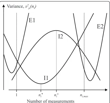
Figure 2 illustrates four principally different cases of how the objective variance function may look as a func-tion of invested resources. At the lower boundary of the choice set, all resources are spent on one unit ofni, and
at the upper boundary on as manynias allowed by the
budget,ni,max. Thus, ifi = s, these two boundaries
cor-respond to allocating as many measurement occasions as possible to one subject, and obtaining measurements at one occasion from as many subjects as possible.
As a general procedure, the optimal ni for a given
budget can be found by comparing the performance obtained: (1) at the lower boundary of the choice set, i.e. usingni= 1, (2) at the upper boundary of the choice set,
i.e. with ni=ni,max, and (3) entering values ofni, if any,
in the interior of the choice set, 1 ≤ ni ≤ ni,max, for which s2μ(ni) = 0.
Thus, examining the properties of the objective func-tion, s2μ(ni), at the boundaries of the choice set is an appropriate first step for identifying the optimal alloca-tion of resources. Provided that the objective funcalloca-tion has one unique minimum, i.e. that the objective function is convex (I1, E1 and E2 in figure 2), a necessary, but also sufficient, condition for the optimum to be internal
Variance, s2
ȝ(ni)
I2
E1
E2
I2
I1
Number of measurements
ni* ni,max
1 ni°
Figure 2Principally different cases of local extremes of the one-variable objective variance function. The boundaries of possible resource investment, i.e. the choice set, are given byni= 1
andni=ni,max. In I1, the variance function has a local minimum at
ni=ni*; this is an interior optimal solution with minimal variance.
For I2, the variance function also has an interior zero derivative, atni
=ni°, but this solution maximizes the variance and is therefore not
(case I1) is that s2μ(ni= 1)<0ands2μ(ni=ni,max)>0.
The exact location of the internal minimum can then be retrieved in a second step. The basic shape of the objec-tive function can be determined by examining its sec-ond-order derivative. If this derivative is positive, the function is convex; if not it is concave (case I2), and the optimal strategy will be at one of the choice set boundaries.
If a convex objective function does not have an internal minimum, as in cases E1 and E2 in figure 2, the optimal strategy is represented by the boundary of the choice set. In case E1, which occurs ifs2μ(ni= 1)>0, the optimal strategy is to setni= 1, that is, collect data from only one
subject (ifi=s), or having only one measurement occasion per subject (ifi=d). Case E2 is characterized by a decreas-ing objective function atni=nmax, i.e.s2μ(ni=ni,max)<0.
In this case, ifi=s, the best choice will be to measure as many subjects as possible and hence only one occasion per subject, or, ifi=d, to collect data for as many occa-sions as possible from only one subject.
Results
Below, procedures for determining optimal sampling strategies are developed using the one-variable substitu-tion approach described above. Procedures will be strati-fied according to the sizes ofaandb, which determine the shape of the cost function (equation (4a)), and
hence the form of the substituted objective
function,s2μ(ni). For each combination of a and b, the objective function is examined, and the boundaries of the choice set determined. Procedures for determining whether the objective function is convex (cases I1, E1 and E2 in figure 2) or concave (case I2) are described where needed. For convex functions, explicit rules are, if possible, developed for when (case I1) and when not (cases E1, E2) the optimal measurement allocation occurs within the choice set. Finally, procedures for identifying an optimal sampling strategy inside the choice set (case I1) are described.
Case A:a= 1,b= 1
In this case, the marginal costs of including another subject or measurement occasion are both independent of the number of previously included subjects and occa-sions. Thus, the cost function is linear at both of these stages.
Case A; substitution and objective function
Witha=b= 1, the budget constraint (equation 4a) can be expressed as:
nd=
R−πs·ns
(πd+cq)·ns (5)
Substituting this expression for nd in equation (3)
gives the corresponding objective function:
s2μ(ns) =
s2
BS
ns +(s
2
BD+s2μWD)·(πd+cq)
R−πs·ns
(6)
Taking the derivative with respect tonsyields:
s2μ(ns) =−
s2
BS
n2
s +(s
2
BD+s2μWD)·πs·(πd+cq) (R−πs·ns)2
. (7)
Setting A= (s2BD+s2μWD)·πs·(πd+cq), equation (7) can be expressed as:
s2μ(ns) =−
s2
BS
n2
s
+ A
(R−πs·ns)2
. (7a)
This one-variable objective function is convex in ns,
since the derivative of equation (7a) is positive for allns
in the choice set.
Case A; boundaries of the choice set
Witha=b= 1, the choice set boundaries in terms ofns
are ns = 1 and ns =ns,max=
R
πs+πd+cq
; the latter
obtained by setting nd = 1 in the budget constraint,
equation (4a), and solving forns.
At ns = 1, equation (7a) takes the form:
s2μ(ns= 1) =−s2BS+
A
(R−πs)2
. Thus, a positive
deriva-tive atns= 1 occurs when:
s2BS< A
(R−πs)2
(8)
This gives a necessary and sufficient condition that the optimal allocation of measurements is obtained with ns
= 1, and hence with nd=nd,max=
R−πs
(πd+cq) measure-ment occasions per subject.
At the other boundary,ns =ns,max=
R
πs+πd+cq, the derivative of the objective function is:
s2μ(ns=ns,max) =
(A−s2BS·(πd+cq)2)·(πs+πd+cq)2
R2·(π
d+cq)2
This derivative is negative only when the first term in the numerator is negative, i.e.A−s2BS·(πd+cq)2<0, or rearranged:
s2BS> (s
2
BD+s2μWD)·πs (πd+cq)
(9)
affordable number of subjects,ns,max=
R
πs+πd+cq, and measure on one occasion for each of these. Notably, condition (9) is independent of the budget R. Also, unlesss2BSis zero, the condition is always valid if πs= 0,
that is if the recruitment of subjects does not lead to any costs. Under case A, this implies that all measure-ment occasions entail the same cost,πd+cq, irrespective
of how they are allocated between subjects. Thus, in this highly simplified case [38,39], the optimal strategy is always to measure on one occasion from each of as many subjects as allowed by the budget.
Case A; optimization inside the choice set
Setting the derivative of the variance function (7a) equal to zero yields:
ns=
R·sBS
A1/2+s
BS·πs
(10)
If this optimal value of ns is an interior solution, i.
e.1≤ns≤
R
πs+πd+cq, the corresponding number of measurement occasions per subject can be obtained by substitution of equation (10) into equation (4a):
nd=
A1/2
sBS·(πd+cq)
(11)
Thus, in this case the optimal number of measure-ment occasions per subject does not depend on the budgetR.
The explicit solution derived above for the optimal set (ns, nd) can lead to non-integer values of one or both
num-bers. Since both are, by nature, discrete, a post-hoc proce-dure may be necessary in which integer sets of (ns, nd)
close to the mathematically derived solution are entered into the budget constraint (equation (4)) to check that they are affordable, and into the objective function (equation (3)) to evaluate their statistical performance. For instance, if an interiornsdetermined by equation (10) is not an
integer, the nearest larger and smaller integers are identi-fied, and for each of those, at least two associated integer values ofndare determined that are larger and smaller
than the value ofndderived by equation (11). The resulting
affordable sets of (ns, nd) are then examined to identify the
one resulting in the smallest mean exposure variance. Table 1 summarizes the derived procedures for opti-mizing cost efficiency in case A, together with proce-dures for the other cases, as derived below.
Case B:a= 1,b≠1
Case B entails constant marginal costs in the recruit-ment of new subjects but either increasing or decreasing marginal costs for organizing measurement occasions.
Case B; substitution and objective function
In case B, the one-variable problem is most easily solved if the objective function is rearranged so that ns is
expressed as a function of nd. From the budget
con-straint, equation (4a),nsis isolated as:
ns=
R
πs+πd·nβd +cq·nd
(12)
The corresponding objective function is:
s2μ(nd) =
(πs+πd·nβd+cq·nd)
R ·(s
2
BS+
(s2
BD+s2μWD)
nd
)(13)
And its derivative:
s2μ(nd) = 1
R·n2
d
·s2BS·(πd·β·nβd+1+cq·n2d)
+ (s2BD+s2μWD)·(πd·(β−1)·nβd −πs)
(14)
The objective function (equation (13)) is always con-vex for b ≥ 2. For 1 <b < 2 it is convex if
s2
BS
(s2
BD+s2μWD)
>−(β−β 2), and for b < 1, convexity
requires s
2
BS
(s2
BD+s2μWD)
<−(β−β 2)(proof, see appendix).
Table 1 Summary of equations, in terms of their numbers in the running text, for identifying the optimal exposure assessment strategy
Combination ofaandb
A:a= 1;b= 1 B:a= 1;b≠1 C:a≠1;b= 1 D:a≠1;b≠1
Budget restriction 5 12 16 NA
Objective variance function; independent variable 6;ns 13;nd 17;ns NA
Derivative of objective function 7 and 7a 14 18 and 18a NA
Condition for choosing lower choice set boundary 8 15 19 NA
Condition for choosing upper choice set boundary 9 NA NA NA
Internalns 10 NA NA NA
Internalnd 11 NA NA NA
If none of these inequalities are fulfilled, the optimal measurement strategy will correspond to one of the choice set boundaries.
Case B; boundaries of the choice set
The choice set boundaries in terms of nd arend = 1
and nd= nd,max. The latter is found by setting ns = 1
in the budget constraint, equation (4a), and rearrange
to get: nβd,max+ cq
πd·
nd,max+πs− R
πd
= 0. This equation
does not have a closed-form solution for nd. In this
case, nd,max can be determined numerically by calcu-lating the cost, c(1, nd), when entering increasing
values ofndin the cost function, equation (4), atns=
1, that is:
c(1,nd) =πs+πd·nβd +cq·nd
nd,maxis then the largest value ofndfor whichc(1,nd)
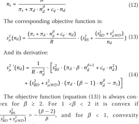
≤ R. Figure 3 illustrates an example of this procedure, for three different combinations of (πs, πd,cq) and two
different levels ofb, which will reappear in the collec-tion of numerical examples.
Atnd= 1, the derivative of the objective function, i.e.
equation (14), is equal to:
s2 μ(1) =
s2
BS·(πd·β+cq) + (s2BD+s2μWD)·(πd·(β−1)−πs)
R ,(14a)
which is positive under the following condition:
s2BS> (s
2
BD+s2μWD)·(πs−πd·(β−1))
πd·β+cq
(15)
Thus, for parameter sets obeying this inequality, the optimal sample allocation is to measure for one
occa-sion on each ofns,max=
R
πs+πd+cq
subjects.
At the other boundary, nd= nd,max, the sign of the derivative of the objective function must be obtained by entering the numerically determined value of nd,max in equation (14). A negatives2μ(nd,max)is then a necessary
and sufficient condition for the optimal measurement strategy to be to choose one subject and measure record from that subject onnd,maxoccasions.
Case B; optimization inside the choice set
The objective function, equation (13), cannot be mini-mized using analytical methods, since s2μ(nd) = 0(cf. equation (14)) does not have a closed-form solution. Thus, a possible interior optimum must be located by entering all values ofndin the interval [1, nd,max] into the objective function and locate the minimal result. The corresponding optimal value of nscan be found by
entering the identified optimal value ofndin equation
(12).
Case C:a≠1,b= 1
In case C, all measurement occasions for a particular subject can be organized at the same cost, while the cost of recruiting additional subjects changes with their numbers.
Case C; substitution and objective function
In case C, the one-variable problem is most easily solved if the objective function is rearranged to expressndas a
function of ns. Isolating nd in the budget constraint,
equation (4a), gives
nd=
R−πs·nαs
(πd+cq)·ns (16)
And hence the objective variance function in terms of nsis:
s2μ(ns) =
s2
BS
ns +(s
2
BD+s2μWD)·(πd+cq)
R−πs·nαs
(17)
Taking the derivate with respect tonsyields:
s2
μ(ns) =−
s2
BS
n2
s
+(s
2
BD+s2μWD)·πs·(πd+cq)·α·nαs−1
(R−πs·nαs)2
(18)
Setting A= (s2BD+s2μWD)·πs·(πd+cq), this can be expressed as:
500
400 500
;a.u.
200 300
nd max=458
al
cost,
c
(1
,nd
)
0 100
d,max
To
ta
Number of measurement occasions, nd
1 10 20 30 40 50 60 70 80 90
Figure 3Numerical determination of the upper boundary of the choice set in case B (a= 1,b≠1). For six different
combinations of unit costs and size of the exponentb, the maximal possible number of measurement occasions, i.e.nd,max, for a single
subject is identified under a budget constraint of 500 (arbitrary units). Squares, rhomboids, and triangles: (πs,πd, cq) = (2, 10, 10), (11,
5.5, 5.5), and (20, 1, 1), respectively. Open and closed symbols:b= 0.50 andb= 1.50, respectively. The value ofnd,maxin each scenario
s2μ(ns) =−
s2BS n2
s
+ A·α·n α−1
s (R−πs·nαs)2
(18a)
It is straightforward to verify that this function is con-vex innsand, hence, has one unique minimum.
Case C; boundaries of the choice set
The choice set boundaries in this case arens= 1 andns
= ns,max. The latter is found by setting nd = 1 in the
budget constraint, equation (4a), and solving forns. This
leads to the equation: nαs,max+ πd+cq
πs ·
ns,max−
R
πs = 0,
which does not have a closed-form solution. Thus, simi-lar to the determination ofnd,maxin case B above,ns,max must be determined by entering increasing values of ns
in the cost functionc(ns, 1) =πs·nsα+ (πd+cq)·nsuntil reaching the largest value ofnsfor whichc(ns, 1)≤R.
At the boundaryns= 1, the derivative of the objective
function, c.f. equation 18a, is:s2μ(1) =−s2BS+ A·α (R−πs)2
.
A necessary and sufficient condition for choosingns= 1,
and hence nd=
R−πs
πd+cq
(cf. equation (16); if necessary
truncated to the nearest smaller integer), is derived by rearranging the inequalitys2μ(1)>0to give:
s2BS< A·α
(R−πs)2
(19)
At the other boundary, ns,max, the sign of the deriva-tive of the objecderiva-tive function must be determined numerically by entering thens,maxidentified above into equation (18a). If the sign is negative,ns,max is the opti-mal number of subjects, and each should be recorded for one occasion.
Case C; optimization inside the choice set
In case C, the equation s2μ(ns) = 0(cf. equation (18a)) has no closed-form solution. Thus, an interior solution to the optimization must be identified by entering allns
in the interval [1,ns,max] into the objective function, i.e. equation (17), and locate the minimal variance. After having identified the optimal ns, the corresponding nd
can be found by solving equation (16).
Case D:a≠1,b≠1
In case D, neithernsnor ndcan be expressed as a
func-tion of the other on basis of the budget constraint. Thus, a one-variable problem cannot be formulated in explicit terms, and, consequently, no analytical expres-sions can be developed, neither for the derivative of the objective function, nor for boundary conditions, nor for possible interior solutions. Therefore, the optimal choice of the number of subjects and measurement occasions has to be identified by means of a numerical procedure, such as the following:
(1) For ns = 1, the cost function, equation (4), is c(1,nd) =πs+πd·nβd +nd·cq.
In this function, increasingnd-values are entered, up
to largest possible value,nd,max, for whichc(1, nd)≤R;
(2) The values (ns, nd) = (1,nd,max1) are entered into
the objective function, equation (3), i.e.
s2μ(1,nd,max 1) =s2BS+
s2
BD+s2μWD
nd,max 1
, and the resulting value
is noted.
(3) These two steps are repeated for ns = 2,
corre-sponding to the cost
functionc(2,nd) =πs·2α+ 2·(πd·nβd +nd·cq), thus obtaining the value ofs2μ(2,nd,max 2)
(4) Subsequent values of s2μ(ns,nd,maxns)are derived using this same procedure for stepwise increasing ns,
until reaching the largest possible ns allowed by the
budget.
(5) By inspecting the set of values of s2μ(ns,nd,maxns), which all entail costs as close as possible to the budget constraint R, the combination ofnsandndoffering the
smallest variance can be identified.
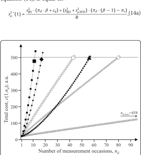
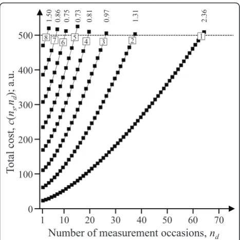
Figure 4 illustrates the numerical procedure for identi-fying the maximal possible value of nd at increasing
values ofns, and the resulting variance of the exposure
mean. Since the values ofns and nd are discrete, and
hence even the corresponding total costc(ns, nd), it may
happen that the optimal measurement strategy does not consume the entire budget R. For instance, the optimal strategy (ns, nd) = (5, 12) identified in figure 4 only
uti-lizes 98.3% of the allowed resources.
Numerical examples
Using the procedures developed above, optimal sam-pling strategies were identified for 225 scenarios repre-senting different combinations of costs and variance components, and different marginal costs of recruiting new subjects and organizing more measurement occa-sions, as expressed througha andb(table 2). Unit costs
πs, πdand cq were selected to illustrate large, medium
As illustrated in table 2, the optimally cost-efficient strategy in many scenarios is to obtain data on one occasion from as many subjects as possible. In particu-lar, this applies whens2BS is“large” relative tos2BDand
s2μWD(table 2c), and even whens2BS is similar to (s2BD
+s2μWD) if πs is also equal to or smaller than (πd+cq)
(table 2b). In these cases, the principle of measuring from as many subjects as possible is valid irrespective of whether cost functions are linear or not, i.e. irrespective of the sizes ofaandb.
Considerable deviations from the principle of collect-ing data from as many subjects as possible do, however, occur; the most extreme examples appearing when s2BS
is “small” relative to s2BD and s2μWDand πsis “large”
compared to (πd+cq)andais“large”(bottom right
cor-ner of table 2a). The combination of a “small” variance between subjects and “large” costs associated with recruiting subjects also leads to the optimal sampling strategy being particularly sensitive to non-linearities in costs. Thus, with (s2BS, s2BD, s2μWD) = (2, 10, 10) and
(πs, πd, cq) = (20, 1, 1), a linear cost function implies an
optimal sampling strategy of (ns, nd) = (13, 9) (table 2a),
while the deviations of a and b from 1 illustrated in table 2 result in optimal strategies (ns, nd) ranging from
(5, 12) to (49, 5), and corresponding variances s2μ
between 0.12 and 0.73. In contrast, with (s2BS, s2BD,
s2μWD) = (20, 1, 1) and (πs, πd, cq) = (2, 10, 10) (table
2c), the most extreme non-linear cost functions lead to sampling strategies, (ns, nd) = (24, 1) and (ns, nd) = (17,
1), which do not deviate much from the optimal strategy in the linear case, (ns, nd) = (22, 1), and only result in
moderate differences in variance.
While not illustrated in table 2, a larger total budget leads to a wider occurrence of the optimal strategy being to collect data on one occasion per subject. Thus, with a budget of 500, 135 of the 225 scenarios illu-strated in table 2 imply that data should be collected according to this principle; if the budget is increased to 1000, this count increases to 139. However, in 3 cases the optimal strategy changes in the opposite direction, i. e. into collecting data on more than one occasion per subject. This was caused by irregularities due to the effect of ns and nd needing to be integers. With a
decreasing budget, one-occasion-per-subject optima get rarer, as expected, but irregularities occur more often.
Even if non-linearities in cost functions may not affect
theprincipleof how to allocate measurements at many
combinations of unit costs and variance components, the size ofa is always important to the eventualsizeof the data set, and therefore to the precision of the even-tual mean exposure estimate. In contrast, the size ofbis only important if the optimal strategy implies, or is close to implying, measurements from more than one occa-sion per subject, that is when s2BS is“small” relative to
s2BDands2μWD(table 2a), but even whens2BS is similar
to (s2BD+s2μWD) ifπs is also larger than (πd+cq) (table
2b). This is an expected result, since the cost of setting up measurement occasions is independent ofbat nd =
1 (cf. equation (4)). Thus, when analyzing whether an intended exposure assessment strategy, constrained by budgets, will lead to a sufficient statistical performance, access to a valid estimate ofais generally more impor-tant than knowing the exact size ofb.
While the size ofb is not always important to size of the optimal data set, the best statistical performance at any specific combination of (s2BS, s2BD, s2μWD) and (πs,
πd, cq) will always be obtained with small sizes ofaand
b; in table 2 exemplified by (a,b) = (0.50, 0.50). This is a reasonable result, since small a and b entail small marginal costs of including more subjects and more measurement occasions.
Although not illustrated in table 2, the effects on sta-tistical performance of deviating from the optimal choice of (ns, nd), but still using the entire budget, were
also investigated. In certain cases, deviations did not lead to any particular reduction of performance. For instance, with (s2BS, s2BD, s2μWD) = (2, 10, 10), (πs,πd,
cq) = (20, 1, 1), and (a, b) = (0.75, 0.75), the optimal
2.36
1.31
0.97
0.81
0.73
0.75
0.86
1.50
400 500
a.u.
3 2 1
4 5 6 7 8
2
0
0
0
0
0
200 300
ost,
c
(
n
s,n
d);
a
100 200
To
tal c
o
1 10
Number of measurement occasions,
n
d20 30 40 50 60 70
0
Figure 4 Numerical procedure for determining the optimal exposure assessment strategy in case D (a≠1,b≠1). For increasing values ofnsas indicated inside the open symbols in each
curve, the maximal number of measurement occasions, i.e.nd,maxns,
allowed by a budget of 500 (arbitrary units) is identified, as marked by open symbols. The resulting statistical performance, i.e.s2
μ(ns, nd,
maxns), is shown above each curve. In the illustrated case, (ns, nd) =
(5, 12) was the optimal allocation.The illustration refers to a scenario with (s2
BS, s2BD, s2μWD) = (2, 10, 10), (πs,πd, cq) = (20, 1, 1), and (a,b)
Table 2 Optimal sampling strategies (ns, nd) and the resulting mean exposure variances2μ(cf. equation (3)) at
different combinations of variance components (s2BS,s2BD,s2μWD; sectionsa-c), unit costs (πs,πd, cq), and exponentsα
andβdescribing the shape of the relationship between costs and number of measurements (cf. equation (4))
a. (s2
BS, s2BD, s2μWD) = (2, 10, 10)
a: 0.50 0.75 1.00 1.25 1.50
(ns, nd) s2μ (ns, nd) s2μ (ns, nd) s2μ (ns, nd) s2μ (ns, nd) s2μ
(πs,πd, cq) b
(2, 10, 10) 0.50 (14, 2) 0.86 (14, 2) 0.86 (10, 3) 0.87 (13, 2) 0.92 (9, 3) 0.96
0.75 (24, 1) 0.92 (13, 2) 0.92 (9, 3) 0.96 (12, 2) 1.00 (8, 3) 1.08
1.00 (24, 1) 0.92 (23, 1) 0.96 (22, 1) 1.00 (11, 2) 1.09 (10, 2) 1.20
1.25 (24, 1) 0.92 (23, 1) 0.96 (22, 1) 1.00 (20, 1) 1.10 (17, 1) 1.29
1.50 (24, 1) 0.92 (23, 1) 0.96 (22, 1) 1.00 (20, 1) 1.10 (17, 1) 1.29
(11, 5.5, 5.5) 0.50 (17, 3) 0.51 (15, 3) 0.58 (11, 4) 0.64 (7, 7) 0.69 (5, 10) 0.80
0.75 (22, 2) 0.55 (14, 3) 0.62 (10, 4) 0.70 (6, 7) 0.81 (6, 6) 0.89
1.00 (39, 1) 0.56 (18, 2) 0.67 (9, 4) 0.78 (8, 4) 0.88 (6, 5) 1.00
1.25 (39, 1) 0.56 (32, 1) 0.69 (14, 2) 0.86 (7, 4) 1.00 (6, 4) 1.17
1.50 (39, 1) 0.56 (32, 1) 0.69 (13, 2) 0.92 (6, 4) 1.17 (5, 4) 1.40
(20, 1, 1) 0.50 (49, 5) 0.12 (27, 7) 0.18 (14, 12) 0.26 (8, 23) 0.36 (6, 28) 0.45
0.75 (52, 4) 0.13 (21, 9) 0.20 (13, 12) 0.28 (8, 19) 0.38 (6, 23) 0.48
1.00 (80, 2) 0.15 (26, 5) 0.23 (13, 9) 0.32 (8, 14) 0.43 (6, 17) 0.53
1.25 (74, 2) 0.16 (27, 4) 0.26 (13, 7) 0.37 (8, 10) 0.50 (6, 12) 0.61
1.50 (134, 1) 0.16 (29, 3) 0.30 (12, 6) 0.44 (9, 6) 0.59 (5, 12) 0.73
b. (s2BS, s 2
BD, s 2
μWD) = (11, 5.5, 5.5)
a: 0.50 0.75 1.00 1.25 1.50
(ns, nd) s 2
μ (ns, nd) s
2
μ (ns, nd) s
2
μ (ns, nd) s
2
μ (ns, nd) s
2 μ
(2, 10, 10) 0.50 (24, 1) 0.92 (23, 1) 0.96 (22, 1) 1.00 (20, 1) 1.10 (17, 1) 1.29
0.75 (24, 1) 0.92 (23, 1) 0.96 (22, 1) 1.00 (20, 1) 1.10 (17, 1) 1.29
1.00 (24, 1) 0.92 (23, 1) 0.96 (22, 1) 1.00 (20, 1) 1.10 (17, 1) 1.29
1.25 (24, 1) 0.92 (23, 1) 0.96 (22, 1) 1.00 (20, 1) 1.10 (17, 1) 1.29
1.50 (24, 1) 0.92 (23, 1) 0.96 (22, 1) 1.00 (20, 1) 1.10 (17, 1) 1.29
(11, 5.5, 5.5) 0.50 (39, 1) 0.56 (32, 1) 0.69 (22, 1) 1.00 (12, 2) 1.38 (9, 2) 1.83
0.75 (39, 1) 0.56 (32, 1) 0.69 (22, 1) 1.00 (12, 2) 1.38 (9, 2) 1.83
1.00 (39, 1) 0.56 (32, 1) 0.69 (22, 1) 1.00 (15, 1) 1.47 (9, 2) 1.83
1.25 (39, 1) 0.56 (32, 1) 0.69 (22, 1) 1.00 (15, 1) 1.47 (8, 2) 2.06
1.50 (39, 1) 0.56 (32, 1) 0.69 (22, 1) 1.00 (15, 1) 1.47 (8, 2) 2.06
(20, 1, 1) 0.50 (134, 1) 0.16 (44, 2) 0.38 (19, 4) 0.72 (11, 6) 1.17 (7, 14) 1.68
0.75 (134, 1) 0.16 (43, 2) 0.38 (18, 4) 0.76 (11, 5) 1.20 (7, 12) 1.70
1.00 (134, 1) 0.16 (42, 2) 0.39 (19, 3) 0.77 (11, 4) 1.25 (7, 9) 1.75
1.25 (134, 1) 0.16 (40, 2) 0.41 (18, 3) 0.81 (10, 5) 1.32 (7, 7) 1.80
1.50 (134, 1) 0.16 (53, 1) 0.42 (20, 2) 0.83 (11, 3) 1.33 (7, 5) 1.89
c. (s2BS, s2BD, s2μWD) = (20, 1, 1)
a: 0.50 0.75 1.00 1.25 1.50
(ns, nd) s2μ (ns, nd) s2μ (ns, nd) s2μ (ns, nd) s2μ (ns, nd) s2μ
(2, 10, 10) 0.50 (24, 1) 0.92 (23, 1) 0.96 (22, 1) 1.00 (20, 1) 1.10 (17, 1) 1.29
0.75 (24, 1) 0.92 (23, 1) 0.96 (22, 1) 1.00 (20, 1) 1.10 (17, 1) 1.29
1.00 (24, 1) 0.92 (23, 1) 0.96 (22, 1) 1.00 (20, 1) 1.10 (17, 1) 1.29
1.25 (24, 1) 0.92 (23, 1) 0.96 (22, 1) 1.00 (20, 1) 1.10 (17, 1) 1.29
1.50 (24, 1) 0.92 (23, 1) 0.96 (22, 1) 1.00 (20, 1) 1.10 (17, 1) 1.29
(11, 5.5, 5.5) 0.50 (39, 1) 0.56 (32, 1) 0.69 (22, 1) 1.00 (15, 1) 1.47 (10, 1) 2.20
0.75 (39, 1) 0.56 (32, 1) 0.69 (22, 1) 1.00 (15, 1) 1.47 (10, 1) 2.20
strategy is to choose (ns, nd) = (21, 9), resulting in a
var-iance of 0.20 (cf. table 2a). However, all strategies with ns in the range between 15 and 32, and corresponding
values ofnd,maxnsranging from 15 to 4 as allowed by the
budget, resulted in variances of 0.22 or less, except for the strategy (30, 4) which gave a variance of 0.23 because it only managed to utilize 92% of the available budget. In other cases, performance was more sensitive to non-optimal choices of (ns, nd). Again using (s2BS,
s2BD, s2μWD) = (2, 10, 10) and (a,b) = (0.75, 0.75), the
optimal strategy with (πs,πd, cq) = (2, 10, 10) is now (ns,
nd) = (13, 2), resulting in a variance of 0.92 (table 2a).
In this case, all strategies allowed by the budget besides the nearest neighbour, (ns, nd) = (12, 2), gave variances
of 1.09 or more, i.e. at least 18% larger than the optimum.
Discussion
As illustrated by the numerical examples in table 2, a large ratio of between-subjects to within-subject var-iance generally implies that the optimal allocation
prin-ciple is to collect data on one occasion from as many
subjects as allowed by the budget. This also applies when between-subjects and within-subject variances are of similar size, unless the unit cost of recruiting subjects is large relative to that of setting up measurement occa-sions. In these cases, non-linearity in the cost functions does not influence the optimal allocation principle; only the eventual size of the data set allowed by budgets. However, at a large relative recruitment cost combined with a small between-subjects to within-subject variance ratio, and in particular if the total budget is also small, the optimal sampling strategy may consist in approach-ing only a few subjects on several occasions each, and the strategy is very sensitive to non-linearities in cost functions. Non-linearities in subject recruitment costs always have a clear influence on thesizeof the optimal data set, while non-linearities in costs for setting up measurement occasions are important only in cases
when the optimal strategy includes multiple measure-ments per subject.
Representativeness
Statistical model
The present study investigated a hierarchical, nested measurement model with three stages as used in a majority of previous studies of the effects of random measurement error on statistical properties and effi-ciency in exposure assessment (e.g. [2,12,26-28]). Even though the application exemplified in the paper refers to subjects, measurement occasions within subjects, and measurement units within occasions, the generic results are applicable also to other sources of exposure variabil-ity that can be described by a hierarchical model. This includes the case of data processing and analysis adding “post-sampling” costs and also some methodological variance to each collected exposure sample, thus modi-fying the sizes of cq (equation (4)) and s2μWD(equation (3)), respectively. Also, the present study addressed, as most other studies, the case of balanced data sampling, i.e. that the same number of measurement units are col-lected during each of the same number of occasions from each subject [23]. While the assumption of a balanced, hierarchical model facilitates mathematical derivation of optimal measurement strategies, cost-effi-ciency needs to be investigated even for more compli-cated models, for instance designs including crossed components [11,29]. In particular, the effects of unba-lancedness, which is probably a very frequent incident in epidemiologic research, need to be addressed in further studies. Unbalancedness has been shown both mathematically [23,57] and empirically [58] to reduce statistical efficiency, and will thus also influence cost-efficiency.
During the last decade, powerful statistical techniques have been developed to analyse exposure variability and its determinants using so-called mixed-effect modelling
[30-33,59]. While mixed model analyses have
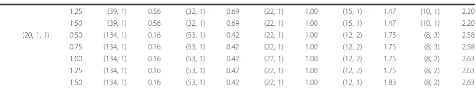
Table 2 Optimal sampling strategies (ns, nd) and the resulting mean exposure variances2μ(cf. equation (3)) at
differ-ent combinations of variance compondiffer-ents (s2BS,s2BD,s2μWD; sections a-c), unit costs (πs,πd, cq), and exponentsαandβ
describing the shape of the relationship between costs and number of measurements (cf. equation (4))(Continued)
1.25 (39, 1) 0.56 (32, 1) 0.69 (22, 1) 1.00 (15, 1) 1.47 (10, 1) 2.20
1.50 (39, 1) 0.56 (32, 1) 0.69 (22, 1) 1.00 (15, 1) 1.47 (10, 1) 2.20
(20, 1, 1) 0.50 (134, 1) 0.16 (53, 1) 0.42 (22, 1) 1.00 (12, 2) 1.75 (8, 3) 2.58
0.75 (134, 1) 0.16 (53, 1) 0.42 (22, 1) 1.00 (12, 2) 1.75 (8, 3) 2.58
1.00 (134, 1) 0.16 (53, 1) 0.42 (22, 1) 1.00 (12, 2) 1.75 (8, 2) 2.63
1.25 (134, 1) 0.16 (53, 1) 0.42 (22, 1) 1.00 (12, 2) 1.75 (8, 2) 2.63
1.50 (134, 1) 0.16 (53, 1) 0.42 (22, 1) 1.00 (12, 1) 1.83 (8, 2) 2.63
predominantly been used to identify exposure targets for effective prevention and intervention, they also represent a challenging opportunity to develop exposure assessment strategies that are both“cheap”and statistically efficient. As an example, several occupational studies have proposed or implemented the idea of estimating full-shift job expo-sures by combining observed or self-reported time propor-tions of tasks in the job with task exposures from a data base [60-65]. In some studies, the task-based estimates appeared easy to obtain and, at the same time, well corre-lated with“true”job exposures (e.g. [66]), while other stu-dies indicate that task-based procedures can also be grossly inefficient [64,65]. Some attention has been given to developing mathematical principles for assessing the statistical performance of task-based exposure modelling [34,67], but no studies have so-far, to our knowledge, addressed if task-based assessment can, indeed, be cost-efficient as compared to direct measurement of job expo-sures, and if so, on which conditions. A similar concern can be raised with respect to other techniques for combin-ing exposure information from different sources into a “hybrid” estimate of some exposure metric [68]. The approach can be statistically informative [68], but might also entail costs to the extent that the trade-off between efficiency and resource consumption is disadvantageous as compared to measuring“true”exposures directly.
Statistical performance criterion
The present study addressed the objective of obtaining a precise estimate of the exposure mean value in a group of subjects (cf. equation (3)), the reason being that pre-cision of the mean is a decisive factor for the usefulness of exposure surveys, and for statistical power in studies comparing conditions and groups. Other measures of statistical performance will, however, be of interest in other types of epidemiologic research, and thus need attention in future cost-efficiency research. A particu-larly important example is the size of bias and/or preci-sion in a regrespreci-sion of outcome on exposure [19-22]. Since both bias and precision can, under a number of assumptions, be expressed as mathematical functions of variance components and the number of measurements [18], it might be possible to develop closed-form solu-tions to the problem of finding optimally cost-efficient measurement strategies, but this has not so-far been pursued. Another example that an exposure assessment strategy may have another purpose than producing a satisfying group exposure mean is standard surveillance of compliance with occupational exposure limits (OEL). First, the assessment focuses on individuals rather than groups, and second, the strategy needs assure that both the individual mean and the probability that single exposure values exceed the OEL is determined with a satisfying certainty [16,17]. Still another relevant mea-sure of statistical performance for several purposes is
the size of the standard reliability coefficient (ICC), i.e. the relationship between exposure variability in data sets with and without (random) measurement error [41].
Obviously, both for regression metrics, exceedance, and ICCs, optimally cost-efficient exposure assessment strategies may deviate from those driven by the objective of obtaining precise exposure means, as illustrated by two studies on optimal measurement allocation in relia-bility studies [69,70].
A particularly challenging situation comes up if the exposure assessment strategy has two simultaneous, yet conflicting objectives. For instance, the researcher may, at the same time, wish to get a precise estimate of a group mean exposure, but also a good estimate of expo-sure variance components between and within workers. This is a likely scenario if the specific exposure variabil-ity of the addressed occupational group isa priori insuf-ficiently known, and the exposure data collection is viewed as an opportunity to get updated data on this variability, together with a documentation of the group mean exposure. Determination of variance components requires, as a minimum, duplicate samples at each stage of the measurement model [5], and this may often not be an optimally cost-efficient strategy if the objective is to get a precise group mean (cf. table 2a-c; cases with nd = 1). Thus, the researcher faces the decision of
whether a certain loss in information on the group mean is an acceptable “price”of getting some informa-tion on exposure variability. While the numerical trade-off between these two types of information, conditional on a restricted budget, may be resolved in future research, the final decision of which sampling allocation to prefer is an issue beyond mathematical procedures.
Recruitment capabilities and cost functions
persuading initially reluctant participants, but also decreasing costs (a<1), as if the first subjects are hard to recruit but their skeptic colleagues, taking after them, will then readily participate. Also, both increasing and decreasing marginal costs for organizing measurement occasions can be envisaged, as if a measurement equip-ment wears down over time and needs to be in place longer to provide a certain amount of data (b>1), or if a subject gets more and more accustomed to measure-ment preparations and thus less time consuming (b<1). As a tentative conjecture, however, considerable devia-tions ofa from 1 are more likely to occur than devia-tions of b. In addition to the need for empirical data describing the shape of cost functions, information is also required concerning thesizeof unit costs for mea-suring at different stages; very little data has been reported in occupational or environmental epidemiology [37,43]. This stands in a striking contrast to the abun-dance of data on variance components for a multitude of occupational and environmental exposures, showing that the size of and relationship between exposure vari-abilities at different stages of measurement, e.g. subjects and occasions within subjects, differ widely between set-tings and exposure agents [3,9-11,25,71,72].
In the present study, optimization procedures were developed using a total cost model including only vari-able cost components (equation (4)). Other studies have addressed even fixed costs, i.e. costs that do not depend on the number of measurements [41,43]. While fixed costs are, under a constrained budget, decisive to the resources left for allocating measurements, they cancel out in the course of the mathematical differentiation associated with the optimization procedure, and thus will not affect the eventual optimal allocation strategy [43]. It is, however, important to notice that the optimi-zation procedures in the present paper all refer to bud-gets where possible fixed costs have already been accounted for.
Analytical vs. numerical optimization
A complete closed-form mathematical solution to cost-efficiency optimization was possible only when cost functions were linear, i.e. (a,b) = (1, 1), and in this case the allocation algorithms were consistent with previous studies [43,44,46,47]. When eitheraorbdeviated from 1, neither the choice set boundaries nor an internal optimum could be explicitly determined, and if both deviated together, all optimization steps had to be per-formed using numerical methods. This suggests that explicit, formal expressions defining cost-efficient mea-surement allocations may only be obtainable if both cost functions and expressions of statistical performance are mathematically very simple. Thus, numerical optimiza-tion procedures might be the only alternative if, for instance, the objective (in casu variance) function
contains not only nested components [11,29], or if the cost model does not express a straight-forward relation-ship with the number of measurements [42]. This points to the idea of basing all optimization on numerical methods and ignore explicit solutions even in those cases where they do exist. However, we believe that mathematical expressions as developed in this paper may still be helpful as a screening tool for deciding whether the optimal strategy needs further (numerical) consideration, or whether it is merely situated at the boundary of the choice set, as in those frequent cases where as many subjects as possible should be measured on one occasion each (cf. table 2).
Sensitivity
The basic cost model
One important result of the present investigation was that for many combinations of unit costs and variance components, non-linear cost functions did not change the general principle stated by a linear model: to mea-sure from as many subjects as possible on one occasion each (cf. table 2). Thus, under these particular circum-stances, the principle of how to optimize exposure assessment was not sensitive to the cost model, even if the eventual size of the data set allowed by budget con-straints was influenced by non-linearities in subject recruitment costs. At other combinations of variance components and unit costs, in particular when between-subject variability was small compared to within-between-subject variability and subject recruitment costs at the same time were large compared to costs for setting up mea-surement occasions, non-linearities did, however, strongly affect both the optimal allocation principle and the eventual statistical performance. While, as men-tioned above, examples of small between- to within-sub-ject ratios of variance are abundant in the literature, relative sizes of unit costs are largely unknown, and thus we do not consider it justified so-far to form an opinion on the actual occurrence of such sensitive scenarios.
Uncertainties in input parameters
small or similar to costs for setting up measurement occasions (table 2). Even the sizeof the eventual data set is robust to changes in exposure variability, as long as recruitment costs are small (table 2). If, however, recruitment unit costs are large, both the allocation and size of the optimal strategy is highly sensitive to the size of variance components, especially if recruitment costs accelerate with the number of subjects (a>1).
Even when closed-form solutions are available for esti-mating the optimal choice of subjects and measurement occasions (equations (10) and (11)), a corresponding analytical expression of the uncertainty of these esti-mates may not be readily available. Optimization using numerical procedures evidently precludes any explicit mathematical representation of uncertainty. Thus, sys-tematic analyses of the stability of optimized strategies to fluctuations in input variables need to be performed by numerical methods. Different approaches may then be viable, including Monte Carlo procedures (e.g. [73]), which will, however, require estimates of the distribu-tions of input variables; and large-scale resampling from empirical distributions as in bootstrapping [74]. Boot-strapping has been used successfully to address uncer-tainty in several occupational studies addressing exposure sampling efficiency [27,53,75], and is especially useful in cases when analytical methods are unavailable [12] or when assumptions underlying the analytical models are probably violated [35,54]. Bootstrap-based analysis of uncertainty has also been used successfully in health economics [76]. However, bootstrapping requires access to - preferably large - empirical data sets that can be used to represent the distributions of necessary vari-ables. In the case of cost-efficiency optimization, this implies that extensive data, not available at present, are needed on unit costs, exponents in the cost function, and exposure variance components.
Deviations from the optimal strategy
For pragmatic reasons, exposure assessments in working life will rarely be carried out as planned (e.g. [37]). Thus, an intended optimal strategy may, in effect, be realized by collecting numbers of measurement units at different stages that deviate from the optimal choice, even if the total budget is still consumed. Presumably, the most likely deviations to occur appear in the form of slight departures from a completely balanced data set; for instance that some measurement occasions fail for some subjects but are compensated by more occasions from others. As noted from the numerical examples (table 2), statistical performance seems to be consider-ably more sensitive to non-optimal strategies at some combinations of variance components, unit costs and cost function exponents than at others. However, this result concerns only non-optimal strategies that are still balanced. The effects of unbalanced reallocations of
measurements, which still consume the allowed budget, need to be determined in future studies. When facing scenarios that will be sensitive to deviations from the optimal strategy, we suggest, however, preparing for likely departures by designing an intentional oversampling.
Comparing cost-efficiencies
Comparing measurement allocations
Some previous studies on cost-efficient data collection have been devoted to comparing two or more alterna-tive measurement strategies with respect to cost and efficiency, rather than identifying an optimal strategy. Thus, Armstrong compared the properties of two differ-ent instrumdiffer-ents for retrieving the same exposure data [40,41], while Lemasters et al. [38] and Shukla et al. [39] devoted their studies to comparing different allocations of measurements using the same instrument. In the two latter studies, probably none of the compared strategies were optimal, but they were meant to represent feasible strategies in terms of e.g. logistics and selection con-straints. The comparison approach to cost-efficiency analysis is considerably easier to deal with from a math-ematical viewpoint than optimization as addressed in the present paper. A mere comparison also allows for both cost and output variance functions that cannot be addressed by analytical optimization procedures. Abstaining from optimization may thus represent a pragmatic level of analysis in cases where the principal objective is to decide for one of a number of possible exposure assessment strategies rather than determining an absolute optimum.
Comparing measurement instruments