Graphical modeling of binary data using the LASSO: a simulation study

(1)

R E S E A R C H A R T I C L E

Open Access

Graphical modeling of binary data using the

LASSO: a simulation study

Ralf Strobl

1*

, Eva Grill

1,2

and Ulrich Mansmann

1

Abstract

Background:Graphical models were identified as a promising new approach to modeling high-dimensional clinical data. They provided a probabilistic tool to display, analyze and visualize the net-like dependence structures by drawing a graph describing the conditional dependencies between the variables. Until now, the main focus of research was on building Gaussian graphical models for continuous multivariate data following a multivariate normal distribution. Satisfactory solutions for binary data were missing. We adapted the method of Meinshausen and Bühlmann to binary data and used the LASSO for logistic regression. Objective of this paper was to examine the performance of the Bolasso to the development of graphical models for high dimensional binary data. We hypothesized that the performance of Bolasso is superior to competing LASSO methods to identify graphical models.

Methods:We analyzed the Bolasso to derive graphical models in comparison with other LASSO based method. Model performance was assessed in a simulation study with random data generated via symmetric local logistic regression models and Gibbs sampling. Main outcome variables were the Structural Hamming Distance and the Youden Index.

We applied the results of the simulation study to a real-life data with functioning data of patients having head and neck cancer.

Results:Bootstrap aggregating as incorporated in the Bolasso algorithm greatly improved the performance in higher sample sizes. The number of bootstraps did have minimal impact on performance. Bolasso performed reasonable well with a cutpoint of 0.90 and a small penalty term. Optimal prediction for Bolasso leads to very conservative models in comparison with AIC, BIC or cross-validated optimal penalty terms.

Conclusions:Bootstrap aggregating may improve variable selection if the underlying selection process is not too unstable due to small sample size and if one is mainly interested in reducing the false discovery rate. We propose using the Bolasso for graphical modeling in large sample sizes.

Background

A common problem in contemporary biomedical research is the occurrence of a large number of variables that accompany relatively few observations. Thus, study-ing associations in high-dimensional data is not straight-forward. Including all variables would result in a highly over parameterized model, computational complexity and unstable estimation of the associations [1]. This methodological problem has been solved for the domain of genomic medicine by using graphical modeling.

Graphical models were identified as a promising new approach to modeling clinical data [2], and thereby the systems approach to health and disease.

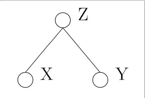
A promising approach to describe such complex rela-tionships is graphical modeling. Graphical models [3] provide a probabilistic tool to display, analyze and visua-lize the net-like dependence structures by drawing a graph describing the conditional dependencies between the variables. A graphical model consists of nodes repre-senting the variables and edges reprerepre-senting conditional dependencies between the variables. In order to under-stand graphical models it is important to underunder-stand the concept of conditional independence. Two variables X and Y are considered conditional independent given Z,

* Correspondence: [email protected] 1

Institute for Medical Informatics, Biometrics and Epidemiology, Ludwig-Maximilians-Universität München, Munich, Germany

Full list of author information is available at the end of the article

(2)

if f(x|y, z) = f(x|z). Thus, learning information about Y does not give any additional information about X, once we know Z.

Beyond association, this method has also been devel-oped for estimating causal effects [4]. Recently, graphical modeling has been outlined as a tool for investigating complex phenotype data, specifically for the visualization of complex associations [5], dimension reduction, com-parison of substructures and the estimation of causal effects from observational data [6]. Until now, the main focus of research was on building Gaussian graphical models for continuous multivariate data following a multivariate normal distribution [7]. A popular way to built Gaussian graphical models are covariance selection methods [8]. These methods are used to sort out condi-tionally independent variables. They aim to identify the non-zero elements in the inverse of the covariance matrix since the non-zero entries in the inverse covar-iance matrix correspond to conditional dependent vari-ables. However, this method is not reliable for high-dimensional data, but can be improved by concentrating on low-order graphs [9].

Another approach to identifying the non-zero ele-ments in the inverse covariance matrix has been pro-posed by Meinshausen and Buehlmann [10]. They propose the Least Absolute Shrinkage and Selection Operator (LASSO) [11] as a variable selection method to identify the neighborhood of each variable, thus the non-zero elements. A neighborhood is the set of predic-tor variables corresponding to non-zero coefficients in a prediction model by estimating the conditional indepen-dence separately for each variable. Meinshausen and Buehlmann showed that this method is superior to com-mon covariance selection methods, in particular if the number of variables exceeds the number of observa-tions. They also proved that the method asymptotically recovers the true graph.

The LASSO was originally proposed for linear regres-sion models and has become a popular model selection and shrinkage estimation method. LASSO is based on a penalty on the sum of absolute values of the coefficients (ℓ1 -type penalty) and can be easily adapted to other

set-tings, for example Cox regression [12], logistic regres-sion [13-15] or multinomial logistic regresregres-sion [16] by replacing the residual sum of squares by the corre-sponding negative log-likelihood function. Important progress has been made in recent years in developing computational efficient and consistent algorithms for the LASSO with good properties even in high-dimen-sional settings [17,18]. The so-called graphical lasso by Friedman et al. [19] uses a coordinate descent algorithm for the LASSO regression to estimate sparse graphs via the inverse covariance matrix. They describe the

connection between the exact problem and the approxi-mation suggested by Meinshausen and Bühlmann [10].

However, the determination of the right amount of penalization for these methods has remained a main problem for which no satisfactory solution exists [20].

The current methodology primarily provides solutions for continuous data. The relationship of binary data is difficult to identify using classical methods. Building binary graphical models for dichotomous data is based on the corresponding contingency tables and log-linear models [21]. The interaction terms are used to control for conditional dependencies. With a growing number of variables model selection becomes computationally demanding and quickly exceeds feasibility, thereby mak-ing the method difficult to adapt to high-dimensional data. For a fully saturated log-linear model one would need2 p parameters, withpbeing the number of vari-ables. A common solution is to reduce the problem to first-order interaction where conditional independence is determined by first-order interaction terms.

The properties of the LASSO for logistic regression have recently been investigated. Van de Geer [22] focused on the prediction error of the estimator and not on variable selection. She proposed a truncation of the estimated coefficients to derive consistent variable selec-tion. Bunea [23] showed the asymptotic consistency of variable selection under certain conditions forℓ1 -type

penalization schemes.

The adaptation of local penalized logistic regression to graphical modeling has been proposed by Wainwright [24]. Under certain conditions on the number of vari-ables n, the number of nodes p and the maximum neighborhood size, the ℓ1 -penalized logistic regression

for high-dimensional binary graphical model selection gives consistent neighborhood selection [24,25]. Wain-wright et al. showed that a logarithmic growth inn rela-tive to p is sufficient to achieve neighborhood consistency. Another new approach is based on an approximate sparse maximum likelihood (ASML) pro-blem for estimating the parameters in a multivariate binary distribution. Based on this approximation a con-sistent neighborhood could be selected and a sensible penalty term can be identified [17].

However, when analyzing high-dimensional categorical data the main problem that there is no rationale for the choice of the amount of penalization controlled by the value of the penalty term for consistent variable selec-tion still remains [20].

(3)

multiple versions are formed, each acting as single learning data for a classification problem. Also, for lin-ear regression it has been shown that bagging provides substantial gains in accuracy for variable selection and classification [26]. This idea has been carried further by Bach [27], resulting in the Bolasso (bootstrap-enhanced least absolute shrinkage operator) algorithm for variable selection in linear regression. Here, the LASSO is applied to several bootstrapped replications of a given sample. The intersection of each of these models leads to consistent model selection.

In this paper we adapted the method of Meinshausen and Bühlmann to binary data and used the LASSO for logistic regression to identify the conditional depen-dence structure. We applied bagging to improve variable selection, hence adapted the Bolasso. Performances are tested on a data set with known structure. This data set was simulated by Gibbs sampling [28]. We also applied graphical modeling methods to real-life data.

Objective of this paper was to examine the perfor-mance of the Bolasso to the development of graphical models for high dimensional binary data with various values for the penalty term and various numbers of bootstraps. We hypothesized that the performance of Bolasso is superior to competing LASSO based methods to identify graphical models. Specifically, the hypothesis was that the choice of the penalty is not critical as long as it is chosen sensibly, i.e. corresponding to a reason-able number of selected varireason-ables.

Methods Data generation

This section presents an approach to simulate high-dimen-sional binary data from a given distribution and dimension by analyzing the results on a data set with known depen-dence structure. This analysis is performed in order to investigate the performance of the proposed methods.

All calculations are done using the statistical comput-ing software R (V 2.9.0) [29].

We propose to generate the data via symmetric local logistic regression models and Gibbs sampling [28] as follows:

(1) Define the p×pmatrix M of odds ratios as:diag

(M)= pii, i =1,..., pwithpiithe baseline odds of variable

X(i)mj_i=pijwithPijas the corresponding odds ratio ofX

(i)

onX(j)and vice versa. (2) Start with k = 0.

(3) Choose starting valuesx(k)= {x1,...,xp) according to

diag(M).

(4) For each iin 1, ...., p generate new x(_ik+1)from a Bernoulli distribution Bp∗_i according to

logitp∗_i=_j₌_imj_i·x(_jk)

(5) Repeat for k = k + 1.After a burn-in phase the x(_ik+1)will reflect the true underlying binary distribution generating X = (X(1) , ..., X(p)) Î {0,1}p We chose a burn-in phase of 5000 iterations.

Real-life data: Aspects of functioning in head and neck cancer patient

We evaluated the method to data measuring aspects of functioning of patients having head and neck cancer (HNC). The data originated from a cross-sectional study with a convenience sample of 145 patients with HNC. The data has previously been used for graphical model-ling and has been published [30].

The patients had at least one cancer at one of the fol-lowing locations: oral region, salivary glands, orophar-ynx, hypopharynx or larynx. Human functioning for each of the patients were assessed using the Interna-tional Classification of Functioning, Disability and Health (ICF) as endorsed by the World Health Organi-zation in 2001 [31]. The ICF provides a useful frame-work for classifying the components of health and consequences of a disease and can be used. According to the ICF the consequences of a disease may concern body functions (b) and structures (s), the performance of activities and participation (d) in life situations depending on environmental factors (e).

Thirty-four aspects of functioning were assessed for each of the patients 12 from the component Body Func-tions, three from the component Body Structure, 15 from the component Activity and Participation and another 4 categories from the component Environmen-tal factors. For better interpretation of the graphs we show the 34 ICF categories together with a short expla-nation in Table 1.

Principles of graphical models

Consider X=(X(1), ...,X(p))Î {0,1}pas a p-dimensional vector of binary random variables. One way to represent the association structure between the elements ofXin a random sample of i.i.d. replicates is an undirected binary graph. A graphG(υ,ε) consists of a finite set of nodesυ, representing the elements of X, and edges εbetween these nodes. Each edge stands for an existing condi-tional dependence between two nodes. Hence, graphical modeling is based on the concept of conditional depen-dence and conditional independepen-dence. To understand graphical models it is fundamental to understand both of these concepts. Two events X and Y are independent, ifP(X ∩Y)=P(X)⋅P(Y) . Two events X and Y are con-ditional independent given Z ifP(X ∩Y|Z)= P(X |Z)

(4)

A concept to describe a graphical model is via the neighborhood of each node. The neighborhood of node

X(a)neais defined as the smallest subset of υ, so thatX

(a)

is conditionally independent of all remaining vari-ables, thus the neighborhood neais defined as:

X(a)⊥

X(i);∀X(i) ∈υ/neanea (1)

Two approaches define the edge setε. First, an edge between x and y exists if and only if both nodes are an element in the opposite neighborhood, i.e. following the AND-rule:

ε=(x,y)|x∈ney∧y∈nex (2)

A less conservative, asymmetrical estimate of the edge set of a graph is given by the OR-rule:

ε=(x,y)|x∈ney∨y∈nex (3)

A different definition of a neighborhood allows for a practical approach. For each node in υconsider optimal prediction of X(a)given all remaining variables. Let baÎ

ℜ(p-1)

be the vector of coefficients for optimal prediction ofX(a). The set of non-zero coefficient is identical to the set of neighbors ofX(a), thus:

nea=

b∈υ :β_ba= 0 (4)

We can regard this as a subset selection problem in a regression setting and to the detection of zero coeffi-cients. The use of shrinkage as the subset selection tool used to identify the neighborhood and to estimate β_ba has become popular in recent years.

Principles of LASSO for logistic regression

Given a set of pexplanatory X(1),...,X(p) and a binary outcome Ythe goal of logistic regression is to model the probabilityπi= p(yi=1|xi)by

log

_π

i 1−πi

=x_iβ⇔πi=

exp(x_iβ)

1 + exp(x_iβ) (5)

The maximum likelihood estimates of bcan be found by setting the first derivative of log-likelihood function equal to zero, thus

∂l(β)

∂β =s(β) = N

i=1 xi

yi−

exp(x_iβ) 1 + exp(x_iβ)

= 0 (6)

The LASSO is a penalized regression technique defined as a shrinkage estimator [11]. It adds a penalty term to equation (6), thus (6) is to be minimized subject to the sum of the absolute coefficients being less than a certain threshold value. Using the absolute values as condition yields shrinkage in some coefficients and simultaneously may set other coefficients to zero as has been shown by Tibshirani [11]. For each choice of the penalty parameter a stationary solution exists often visualized as a regularization path, i.e. the penalized coefficients over all penalty terms. LASSO reduces the variation in estimatingb. Formally, the penalized logistic regression problem is to minimize:

N

i=1 xi

yi−

exp(x_iβLASSO₎ 1 + exp(x_iβLASSO₎

+λ j

βLASSO

(j) (7)

Table 1 Short description of the ICF categories used for the graphical models on the HNC data

ICF Code

ICF Code description

b130 Energy and drive functions

b280 Sensation of pain

b310 Voice functions

b320 Articulation functions

b340 Alternative vocalization functions

b440 Respiration functions

b450 Additional respiratory functions

b460 Sensations associated with cardiovascular and respiratory functions

b510 Ingestion functions

b515 Digestive functions

b530 Weight maintenance function

b710 Mobility of joint functions

d175 Solving problems

d310 Communicating with - receiving - spoken messages

d315 Communicating with - receiving - nonverbal messages

d330 Speaking

d335 Producing nonverbal messages

d350 Conversation

d360 Using communication devices and techniques

d550 Eating

d560 Drinking

d570 Looking after one’s health

d720 Complex interpersonal interaction

d760 Family relationship

d770 Intimate relationship

d850 Remunerative employment

d920 Recreation and leisure

s320 Structure of mouth

s430 Structure of respiratory system

s710 Structure of head and neck region

e125 Products and technology for communication

e225 Climate

e310 Immediate family

(5)

A mathematically equivalent expression of this blem is the formulation as a constrained regression pro-blem, that is minimizing

N

i=1 xi

yi−

exp(x_iβLASSO₎ 1 + exp(x_iβLASSO₎

(8)

subject to

j βLASSO

(j) <t. In this paper, the variables are first standardized to zero mean and variance one. The penalty termt can be used to control the number of predictors, i.e. the size of the neighborhood.

Binary graphical model using single LASSO regressions The first method considered here to construct graphical models is based on an optimal penalty term to identify an optimal neighborhood. We consider three procedures for selecting optimal penalty, namely cross-validation (CV), Akaike Information Criteria (AIC) and Bayesian Information Criteria (BIC). These approaches have although been suggested in recent publications by Vial-lon [32] and Wang [33]. The first one is proposed by

Goeman in the context of Cox regression [34], while the latter two are computational more efficient and well-known classical tools. BIC has shown to be superior as suggested by Yuan and Lin and demonstrated superior performance through simulation studies in Gaussian graphical modes [35,36]. Other possible approaches include the methods by Wainwright [24] and Banerjee [17] which control the rate of falsely detected edges in the graph. However, these penalties are too conservative as outlined in Ambroise et al. [37]. The LASSO and cross-validation are calculated using the efficient gradi-ent-ascent algorithm as proposed by Goeman and are implemented in the‘penalized’package [38].

For all possible penalty terms, the performance of the resulting models is assessed either by cross-validation, AIC or BIC. The algorithm to identify a binary graphical model then proceeds as follows:

1. Estimate the coefficients_βˆLASSO_{in local penalized} logistic regression models using each variable as out-come and the remainder as predictors for eachX(i)

(6)

2. For each variable adefine the neighborhoodne∗_aas the set of variables b corresponding to non-zero penalized coefficientsβˆa

b :ne∗a ={b∈υ:βˆba= 0}. 3. Define the set of conditional relationships (the edge set) E as:E={(a,b)|a∈ne∗_b∨b∈ne∗_a}.

Binary graphical model using bolasso

Another method to construct binary graphical models is based on the Bolasso algorithm which takes advantage of bootstrap aggregating. Bootstrap aggregating, also called‘bagging’, generates multiple versions of a predic-tor, e.g. a coefficient in a generalized linear model, or classifier. It constitutes a simple and general approach to improve an unstable estimatorθ(X) with X being a given data set. Bagging is based on the concept of resampling the data {(yn , xn), n = 1,..., p} by drawing

new pairsy∗_n,x∗_n with replacement from theporiginal data pairs. For simple classification the bootstrap aggre-gating algorithm proceeds as follows:

(1) Generate a bootstrap sample b*with replacement from the original data. Repeat this processBtimes.

(2) For each data sampleb* calculate the classifierθ* (b*).

(3) Count the times an object is classified

μx= i=1..B

θ∗ i

b∗_i_.

(4) Define the set of classified objects asS = {y:μy ≥

πcut} with 0≤πcut≤1.

Using Bolasso as a basis, we can now construct gra-phical models. The algorithm proceeds as follows:

(1) Generate a bootstrap sample b*with replacement from the original data. Repeat this process B times.

(2) For each b*, estimate the coefficients _βˆLASSO_in local penalized logistic regressions using each variable as outcome variable and the remainder as predictors for a penalty termt.

(3) For each variableadefine the neighborhoodne∗_aas the set of variables b corresponding to non-zero pena-lized coefficientsβˆa

b:ne∗a={b∈υ:βˆba= 0}.

(4) Calculate the percentage variablebis in the neigh-borhood ofain each bootstrap sampleb*asμa_b.

(5) Define the neighborhood of variable a as: ne∗_a ={b|μa

b≥πcut}

(6) Define the set of conditional relationships (the edge set) E as:E={(a,b)|a∈ne∗_b∨b∈ne∗_a}.

Three parameters have to be chosen here:

•B: number of bootstraps

•t: penalty parameter

•πcut: cut-off value for the definition of neighborhood

In our study, we investigated the influence of these parameters for different sample sizes in a study based on simulated data as described earlier. We also

considered using a cross-validated penalty as a basis for the Bolasso and refer to this approach by Bolasso-CV.

Assessment of performance

We analyzed the performance of the methods by com-paring the identified structure with a predefined known structure. Thus, each edge yielded by one method can be either correct or incorrect. A falsely identified (false positive) edge is an edge which is identified by one or both of the two methods but does not exist in the pre-defined structure. A falsely not identified (false negative) edge is an edge which is not identified by one or both of the two methods but does exist in the predefined structure. A correctly identified (true positive) edge is an edge which is identified by one or both of the two methods and which exists in the predefined structure. Likewise, a true negative edge is an edge correctly iden-tified as missing.

We report the Structural Hamming Distance (SHD) and the Youden index (J). The SHD between two graphs is the number of edge insertions or deletions needed to transform one graph into the other. Thus, the number of changes needed to transform the graphical model identified by one or both of the two methods to the known structure defined by the matrix M. The SHD measures the performance of LASSO and Bolasso by counting the number of false positive and false negative edges.

It may occur that bagging causes the exclusion of all edges yielding a SHD equal to the number of true edges. This might reduce the error rate, but an empty model without edges is not always desirable, even if it has a low error rate. In order to assess both, the ability to find true positive and true negative edges, the Youden Index is more appropriate.

The Youden index is a function of the sensitivity (q) and the specificity (p) of a classifier and is defined as:

J=q+p−1 (9)

Sensitivity is the proportion of true positive edges among all identified edges and specificity the proportion of true negative edges among all not identified edges.

Smaller values of the SHD indicate better choice, as do larger values of the J. Thus, a choice is to be pre-ferred that yields small SHD at large J values.

(7)

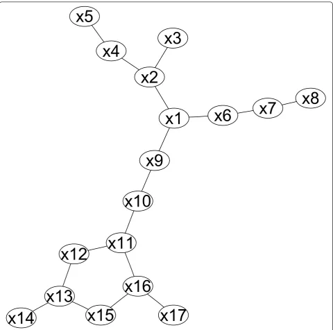
Figure 2 corresponds to a particular matrix of odds ratios, e.g. a smaller model with only 6 variables can be expressed by the matrix M:

M=

⎛ ⎜ ⎜ ⎜ ⎜ ⎜ ⎜ ⎝

1 2 2 1 1 1 2 1 1 2 1 1 2 1 1 2 1 1 1 2 2 1 1 1 1 1 1 1 1 1 1 1 1 1 1 1

⎞ ⎟ ⎟ ⎟ ⎟ ⎟ ⎟ ⎠

We chose the penalty term to be either cross-vali-dated, AIC or BIC optimal or to correspond to a certain neighborhood size ranging from one to the maximum neighborhood size, i.e. lÎ(1,2,...,18) in the original data. In addition, we varied the number of bootstrap repli-catesB Î(40,80,120,160,200), the threshold for a vari-able to be included in a neighborhood πcut Î

(0.90,0.95,0.99,1.00) and the sample size n Î

(50,100,200,500,1000). Usually,Blies in the range of 50. However, the best choice is not clear, e.g. Bach

x1

x2

x3

x4

x5

x6

x7

x8

x9

x10

x11

x12

x13

x14

x15

x16

x17

(8)

investigated alsoB= 256, and may be important as the method itself is unstable. The choice of thresholds was also motivated by the work of Bach who proposed the soft Bolasso with a threshold of 0.90 as opposed to the Bolasso with a threshold of 1.00. We chose a wide range of values for B, thresholds and sample size to simulta-neously study the performance of B and thresholds in small samples and in big samples. Ideally, for a sample size of 1000 the methods should perform with negligible error. In order to estimate model performances depen-dent on the parameters πcut, Bandland the interaction

between πcut and l we calculated generalized linear

models with either SHD or J as outcome variable.

Result

Simulations results

We calculated the Structural Hamming Distance and Youden Index for the simulation setting for each combi-nation of B, πcutand l. We give the detailed results in

table form in the electronic supplement (see additional file 1 and additional file 2: Summary statistics for the simulation study). Using generalized linear model yielded the following optimal regularization for minimal SHD:πcut =0.90,B= 200 andl=5 . For a maximal J a

larger neighborhood size is preferred: πcut= 0.90,B=

200 andl =10. It turned out, that the number of boot-strap replicatesBhas the least influence on model per-formance with higherBperforming slightly better.

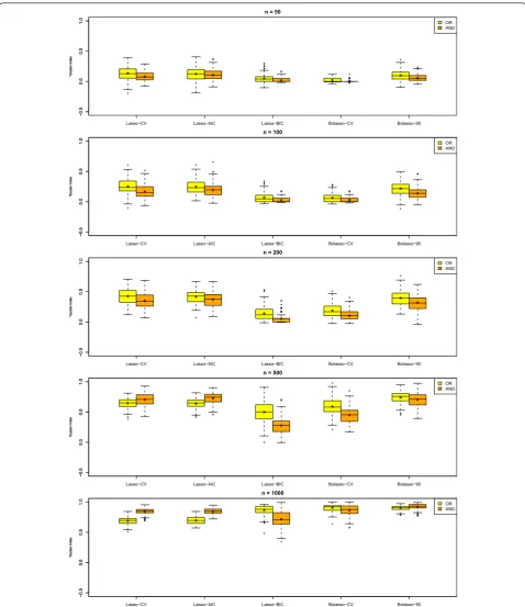
We give a summary of the results for SHD in Figure 3 and for J in Figure 4 for varying sample size. The figures show box plots for all methods, namely the Lasso-CV, the Lasso-AIC, the Lasso-BIC, the Bolasso-CV and the Bolasso with optimal neighborhood size andπcut=0.90,

the Bolasso-90. For each method we applied two differ-ent neighborhood definitions corresponding to the AND-rule and to the OR-rule. In the box plots * marks the mean performance.

Considering SHD as the main outcome renders Lasso-CV and Lasso-AIC as clearly inferior. For smaller sam-ple sizes Lasso-BIC, Bolasso-CV and Bolasso-90 reject almost or all edges eading to a null model with SHD equal to 19. For sample sizes greater than 500 Bolasso-CV and Bolasso-90 are clearly superior to Lasso-BIC. Additionally, for each approach the AND-rule was superior to the OR-rule for most sample sizes.

A similar result can be seen when considering the Youden Index with the exception that Lasso-CV and Lasso-AIC are real contenders here, as they are not as conservative as the others, such gaining performance regarding sensitivity.

HNC data

Using these results we applied the method to the HNC data set using both the AND- and OR-rule. We give the

results for the CV, the AIC and the BIC optimal penalty and for the Bolasso with a cut of 90%, 200 bootstraps and a neighborhood size of 5 (for optimal SHD), resp. 10 (for optimal J) in Figure 5 and 6. The color of the nodes correspond to the different ICF components: ICF categories from the component Body function are orange, Body structure white, Activities and participa-tion blue and Environmental factors green. The full descriptions of the ICF categories are in Table 1.

In all models similar aspects can be seen. The CV and AIC optimal penalty term leads to a very complicated model, while the BIC criteria yielded reasonable results in terms of interpretability. The Bolasso-90 is the most conservative approach while using Bolasso-CV yielded similar results than the Lasso-BIC.

As a case in point, we describe the model for the Bolasso-90 with a neighborhood size of 10, i.e. the model with the highest performance regarding the You-den Index.

Similar to Becker et al. [30] we identified a circle-like association around the speaking capability, i.e. between d330 Speaking, b310Voice functions, b320Articulation functions, s320 Structure of mouth, b510Ingestion func-tions, d350 Conversation, d360 Using communication devices and techniques. The latter had further associa-tions to e125Products and technologies for communica-tionand d920Recreation and leisure. The category s320

Structure of mouth had a meaningful connection to d560 Drinking which was further connected to d550

Eating. Furthermore, b510Ingestion functions had an association to b280Sensation of pain. On the left side of the graph we have a group around respiration functions, namely b440 Respiration functions, b450 Additional respiratory functions, b460Sensations associated with cardiovascular and respiratory functionsand s430 Struc-ture of respiratory system. A further like path could be visualized between the categories d335 Producing non-verbal messages, d315Communicating with receiving -nonverbal messages, d310Communicating with - receiv-ing - spoken messages, d720Complex interpersonal inter-action, d570Looking after one’s health and b130Energy and drive functions. The big circle is closed by the con-nection of b130 and d920Recreation and leisure.

Many of these association structures were also present in the original work and are discussed in detail there [30].

Discussion

(9)

● ● ● ● ●● ●● 0 102 03 04 05 0

n = 50

Str

uctur

al Hamming Distance

* * _* * ● ● ● ● ● ● ● ● ● ● ● ● ● ● ● ●●● ● ● ●●● ● ● ●● ● ●● ● ●● ● ● ●● ● ● ●● ●●● ● ● ● ● ● ● ● ●● ● ● ● ● ● ● ● ● ●● ● ● ● ●●● ● ●● ● ●● ● ● ● ● ● ● ● ●● ● ● ● ● ● ● ● ● ●● ● ●●● ●●●● ● ● ● ●● ● ● ● ●● ● ● ● ● ●●●●● ● ● ● ● ● ●● ● ● ● ●● ● ● ● ● ● ●●● ● ●●● ● ● ● ●●●● ● ● ● ●●● ● ●● ● ●●● 0 102 03 04 05 0 Str uctur

al Hamming Distance *

*

* * *

Lasso−CV Lasso−AIC Lasso−BIC Bolasso−CV Bolasso−90

OR AND ● ● ● ● ● ● ● ● ● ● ● ● ● ● ● ● ● ● ●● ● ● ● ● ● ● ● ● ● ● ● ● ● ●● ● ● 0 102 03 04 05 0

n = 100

Str

uctur

al Hamming Distance

* * * * * ●●● ● ● ●● ● ● ● ● ● ●●●●●●●●● ● ● ●●● ● ● ● ● 0 102 03 04 05 0 Str uctur

al Hamming Distance * *

* * *

OR AND ● ● ●● ● ● ● ● ●●● ● ●● ● ● 0 102 03 04 05 0

n = 200

Str

uctur

al Hamming Distance

* * * * * ● ● ● ● ● ● ● ● ● ● ● ● ● ● ● ● ●● ● ●● ● ● ●● ● 0 102 03 04 05 0 Str uctur

* * *

OR AND ● ● ● ● ● 0 102 03 04 05 0

n = 500

Str

uctur

al Hamming Distance

* * * * * ● ● ● ●● ● ● ● 0 102 03 04 05 0 Str uctur

* _*

*

OR AND ● ● ●●● ● ● ● ● ● ●●● 0 102 03 04 05 0

n = 1000

Str

uctur

al Hamming Distance

* * * * * ● ● ● ● ● ● ● ● ●●● ●● 0 102 03 04 05 0 Str uctur

* _*

*

OR AND

(10)

● ● ● ● ● ● ● ● − 0.5 0.0 0.5 1.0

n = 50

Youden Inde x * * _* * * ●● ●● ● ● ● ● ●● ● ●●● ●●●●●● ● ●● ● ●● ●● ● ● ●●●●●● ●● ●●● ● ● ●● ●● ● ●● ●● ● ● ● ● ●●●● ●● ● ● ●● ● ● ●● − 0.5 0.0 0.5 1.0 Youden Inde x * * _* * *

OR AND ● ● ● ●● ● ● ● ●● ● − 0.5 0.0 0.5 1.0

n = 100

Youden Inde x * * * * * ● ● ● ● ●●● ●●● ●●● − 0.5 0.0 0.5 1.0 Youden Inde x * * * * *

OR AND ● ●● ● ● ● − 0.5 0.0 0.5 1.0

n = 200

Youden Inde

x * _*

* * * ●● ● ●● ● ● ● ● ●● ● ● ● ● ● ● − 0.5 0.0 0.5 1.0 Youden Inde x * * * * *

OR AND ● ● ● ● ● ● ● ●●● − 0.5 0.0 0.5 1.0

n = 500

Youden Inde x * * * * * ●● ●●● ● − 0.5 0.0 0.5 1.0 Youden Inde x * * * * *

OR AND ● ● ● ● ● ●●● − 0.5 0.0 0.5 1.0

n = 1000

Youden Inde x * * * * * ●●● ●● ●● ● ●● ● ● ● ●● ● ●● − 0.5 0.0 0.5 1.0 Youden Inde x * * * * *

OR AND

(11)

parameters, and are susceptible to small changes in the data set [6]. Interestingly, we found that using a BIC penalty and Bolasso were both able to correctly identify predefined existing dependency structures.

We have analyzed several LASSO based methods to derive graphical models in the presence of binary data and compared their performance in detecting known dependency structures. All methods are taking advan-tage of penalized logistic regression models as a tool to identify the explicit neighborhoods. We could show that bootstrap aggregating can substantially improve the per-formance of model selection, especially in the case of large samples. Arguably, LASSO is inferior in certain situations because in a given LASSO coefficient path the optimal solution might not exist. A LASSO coefficient path is given by the coefficient value of each variable over all penalty terms. In contrast, bagging opens the window for a whole class of new models, because it selects all variables intersecting over the bootstrap sam-ples. The intersection itself must not be a solution in any of the bootstrap samples.

In LASSO, the choice of the penalty often determines the performance of the model. Thus, the correct choice of the penalty term is important. However, in our study, the initial choice of penalization had surprisingly little impact on the performance of the model if bagging was applied and the penalty was chosen in sensibly. Similar results have been obtained with stability selection [20]. Stability selection is also based on bootstrap in combi-nation with (high-dimensional) selection algorithms. It applies resampling to the whole LASSO coefficient path and calculates the probability for each variable to be selected when randomly resampling from the data.

In our study, bagging largely improved the perfor-mance of LASSO, but only by reducing the number of false positive and false negative edges. This, however, might lead to a conservative and underspecified model with a low number of edges, if any, especially in small samples.

(12)

arbitrary choice will determine the size of the graphical model. Reducing the cut-off value would include more variables at the expense of a higher false positive rate.

This study illustrates that in graphical modeling, it is essential not only to control the number of false positive and false negative edges but also the ability of a method to identify true positive edges.

Conclusion

Bootstrap aggregating improves variable selection if the underlying selection process is not too unstable, e.g. due to small sample sizes. These properties have been shown on simulated data using various parameters. As a consequence, we propose using Bolasso for graphical modeling in large sample size cases as a real contender to the classical neighborhood estimation methods.

Additional material

Additional file 1: The table in the electronic supplement gives the exact numbers of the performances of each model. The table gives

summary statistics (mean, median, standard deviation, minimum and maximum) for the Structural Hamming Distance.

Additional file 2: The table in the electronic supplement gives the exact numbers of the performances of each model. The table gives summary statistics (mean, median, standard deviation, minimum, and maximum) for the Youden Index.

Acknowledgements

The authors thank Emmi Beck for manuscript revision and Sven Becker for providing the data for the real-data study.

This study was funded by the German Research Foundation (Deutsche Forschungsgemeinschaft) (GR 3608/1-1).

Author details

1_{Institute for Medical Informatics, Biometrics and Epidemiology,}

Ludwig-Maximilians-Universität München, Munich, Germany.2_{Faculty of Health and} Nursing Sciences, West Saxon University of Applied Sciences, Zwickau, Germany.

Authors’contributions

RS computed the study; EG and UM contributed to the design of the study; all authors contributed to the analysis and writing. All authors read and approved the final manuscript

(13)

Competing interests

The authors declare that they have no competing interests.

Received: 19 August 2011 Accepted: 21 February 2012 Published: 21 February 2012

References

1. Breiman L:Heuristics of Instability and Stabilization in Model Selection.

Ann Stat1996,24:2350-2383.

2. Tsai CL, Camargo CA Jr:Methodological considerations, such as directed

acyclic graphs, for studying“acute on chronic”disease epidemiology:

chronic obstructive pulmonary disease example.J Clin Epidemiol2009,

62:982-990.

3. Edwards D:Introduction to Graphical ModellingNew York: Springer; 2000. 4. Hernan MA, Robins JM:Instruments for causal inference: an

epidemiologist’s dream?Epidemiology2006,17:360-372.

5. Strobl R, Stucki G, Grill E, Muller M, Mansmann U:Graphical models illustrated complex associations between variables describing human

functioning.J Clin Epidemiol2009,62:922-933.

6. Kalisch M, Fellinghauer BA, Grill E, Maathuis MH, Mansmann U, Buhlmann P, Stucki G:Understanding human functioning using graphical models.

BMC Med Res Methodol2010,10:14.

7. Wong F, Carter CK, Kohn R:Efficient estimation of covariance selection

models.Biometrika2003,90:809-830.

8. Dempster AP:Covariance Selection.Biometrics1972,28:157-175. 9. Wille A, Bühlmann P:Low-order conditional independence graphs for

inferring genetic networks.Stat Appl Genet Mol Biol2006,5:1-32.

10. Meinshausen N, Buehlmann P:High-dimensional graphs and variable

selection with the Lasso.Ann Stat2006,34:1436-1462.

11. Tibshirani R:Regression shrinkage and selection via the lasso.J R Stat Soc

1996,58:267-288.

12. Tibshirani R:The lasso method for variable selection in the Cox model.

Stat Med1997,16:385-395.

13. Genkin A, Lewis DD, Madigan D:Large-Scale Bayesian Logistic Regression

for Text Categorization.Technometrics2007,49:291-304.

14. Lokhorst J:The LASSO and Generalised Linear ModelsHonours Projects Department of Statistics. South Australia, Australia: The University of Adelaide; 1999.

15. Shevade SK, Keerthi SS:A simple and efficient algorithm for gene

selection using sparse logistic regression.Bioinformatics2003,

19:2246-2253.

16. Krishnapuram B, Carin L, Figueiredo MA, Hartemink AJ:Sparse multinomial

logistic regression: fast algorithms and generalization bounds.IEEE Trans

Pattern Anal Mach Intell2005,27:957-968.

17. Banerjee O, El Ghaoui L, d’Aspremont A:Model Selection Through Sparse Maximum Likelihood Estimation for Multivariate Gaussian or Binary

Data.J Mach Learn Res2008,9:485-516.

18. Rothman AJ, Bickel PJ, Levina E, Zhu J:Sparse permutation invariant

covariance estimation.Electronic Journal of Statistics2008,2:494-515.

19. Friedman J, Hastie T, Tibshirani R:Sparse inverse covariance estimation

with the graphical lasso.Biostatistics2008,9:432-441.

20. Meinshausen N, Buehlmann P:Stability Selection.Journal of the Royal Statistical Society Series B2010,72:417-473.

21. Agresti A:Categorical Data AnalysisNew Jersey: Wiley; 2002.

22. van der Geer SA:High-dimensional generalized linear models and the

Lasso.Ann Stat2008,36:614-645.

23. Bunea F:Honest variable selection in linear and logistic regression

models viaℓ1 andℓ1 +ℓ2 penalization.Electronic Journal of Statistics

2008,2:1153-1194.

24. Wainwright MJ, Ravikumar P, Lafferty JD:High-dimensional graphical

model selection using l1-regularized logistic regression.Advances in

Neural Information Processing Systems2007,19:1465-1472.

25. Ravikumar P, Wainwright MJ, Lafferty JD:High-dimensional Ising model

selection using_ℓ1-regularized logistic regression.Ann Stat2010,

38:1287-1319.

26. Breiman L:Bagging predictors.Mach Learn1996,24:123-140. 27. Bach FR:Bolasso: Model consistent lasso estimation through the

bootstrap.preprint2008.

28. Robert CP, Casella G:Monte Carlo Statistical Method.New York: Springer;, 2 2004.

29. R Development Core Team:R: A Language and Environment for

Statistical Computin.Vienna, Austria: R Foundation for Statistical

Computing; 2009.

30. Becker S, Strobl R, Cieza A, Grill E, Harreus T, Schiesner U:Graphical modeling can be used to illustrate associations between variables

describing functioning in head and neck cancer patients.J Clin Epidemiol

2011.

31. World Health Organization:International Classification of Functioning,

Disability and Health: ICF.Book International Classification of Functioning

Disability and Health: ICFCity: WHO; 2001, (Editor ed.^eds)..

32. Viallon V, Banerjee O, Rey G, Jougla E, Coste J:An empirical comparative study of approximate methods for binary graphical models; application to the search of associations among causes of death in French death

certificates.2010, http://arxiv.org/pdf/1004.2287.

33. Wang P, Chao DL, Hsu L:Learning networks from high dimensional

binary data : An application to genomic instability data.2010, http://

arxiv.org/pdf/0908.3882.

34. Goeman JJ:L1 penalized estimation in the Cox proportional hazards

model.Biom J2009,52:70-84.

35. Gao X, Pu DQ, Wu Y, Xu H:Tuning parameter selection for penalized

likelihood estimation pf inverse covariance matrix.2010, http://arxiv.org/

pdf/0909.0934.

36. Yuan M, Lin Y:Model selection and estimation in the Gaussian graphical

model.Biometrika2007,94:19-35.

37. Ambroise C, Chiquet J, Matias C:Inferring sparse Gaussian graphical