Gabriel Caloz & Monique Dauge, Editors
TOWARDS A SELF-ADAPTIVE PARAMETERIZATION
FOR AERODYNAMIC SHAPE OPTIMIZATION
R´
egis Duvigneau
1, Badr Abou El Majd
1and Jean-Antoine D´
esid´
eri
1Abstract. In parametric shape optimization, results usually depend on the choice of the parame-terization. In order to reduce this critical dependency, a self-adaptive parameterization methodology is developed, that adapts an initial and perhaps na¨ıve parameterization to the problem studied, on the basis of a first approximation of the optimum shape. The proposed approach is studied in the framework of the B´ezier curve representation and the Free-Form Deformation (FFD) approach. It is first applied to a geometrical arc reconstruction problem and then to a three-dimensional shape optimization problem in aerodynamics.
R´esum´e. En optimisation de forme param´etrique, les r´esultats d´ependent g´en´eralement du choix de la param´etrisation. Afin de r´eduire cette d´ependance critique, une m´ethode de param´etrisation auto-adaptative est d´evelopp´ee, qui permet d’adapter au probl`eme ´etudi´e une param´etrisation initiale et peut-ˆetre na¨ıve, sur la base d’une premi`ere approximation de la forme optimale. Cette approche est ´etudi´ee dans le cadre d’une repr´esentation par courbes de B´ezier et par l’approche des boˆıtes englobantes. Elle est appliqu´ee tout d’abord `a un probl`eme g´eom´etrique de reconstruction d’un arc, puis `a un probl`eme d’optimisation de forme tridimensionnelle en a´erodynamique.
Introduction
In parametric shape optimization, a geometrical shape representation has to be chosena priori, such as the use of B´ezier curves for instance. This task is called parameterization. This choice determines a subspace in which the search of the optimum shape is performed. This strategy has several advantages, such as:
• the reduction of the dimension of the problem, that is mandatory for stochastic optimization for
in-stance ;
• the control of the smoothness of the shapes, that is necessary for numerical calculations and most
realistic applications.
However, this strategy drastically reduces the set of shapes that can be reached by the optimization procedure. Then, the optimum shape found usually depends on the parameterization. The use of a parameterization that is not well adapted to the optimization problem can yield a low fitness optimum shape. Hence, in order to reduce this critical dependency, a self-adaptive parameterization methodology is developed, that adapts an initial and perhaps na¨ıve parameterization to the problem studied, on the basis of a first approximation of the optimum shape.
1 INRIAOpaleProject-Team, 2004 route des lucioles, BP 93, 06902 Sophia-Antipolis, FRANCE (www-sop.inria.fr/opale)
c
EDP Sciences, SMAI 2007
1.1.
B´
ezier curve
One proposes to modify some characteristics of the parameterization to adapt it to the particular problem studied. For instance, consider an airfoil shape described by a B´ezier curve:
P(t) = n
X
i=0
Bin(t)Pi, (1)
where t ∈ [0,1] and {Bi
n}i=0,...,n are the Bernstein polynomials of degreen. The coordinates of the control pointsPi= xyiican be considered as design variables during the optimization procedure. Since an airfoil is a rather thin body, only ordinates{yi}i=0,...,n are usually taken into account during the optimization, whereas abscissae{xi}i=0,...,nare frozen. Then, one proposes to consider the abscissae{xi}i=0,...,n as adaption variables that can be used to control the characteristics of the parameterization [3].
Initially, the abscissae{xi}i=0,...,ncan be uniformly distributed. Once a first approximation of the optimum shape has been found by modifying the ordinates {yi}i=0,...,n, new abscissae{xi}i=0,...,n are defined, that are better adapted to the problem, before a second optimization step is carried out. Actually, the abscissae are defined in such a way that an adaption cost functional is minimized, that measures the uneffectiveness of the current parameterization, with the constraint that the current shape remains unaltered. This constraint is introduced to benefit from the optimization path already performed.
For a given set of abscissae{xi}i=0,...,n, consider the ordinates {yi}i=0,...,n for which the shape is the least-squares approximation of the current shape. Then, the new abscissae{xi}i=0,...,nare chosen in order to minimize the total variation of the corresponding ordinates{yi}i=0,...,n:
T V({yi}) =
n
X
i=1
|yi−yi−1| ≈ Z 1
0
|y′(t)|dt, (2)
where y(t) is interpolating the control points. This criterion is introduced to regularize the control points polygon. This choice is justified by the fact that the optimization process yields a highly irregular control points polygon [2].
1.2.
Free-Form Deformation (FFD)
For complex three-dimensional problems, such as those encountered in aerodynamics, the Free-Form De-formation (FFD) approach [6] is adopted. It consists in defining a lattice embedding the shape and a local coordinate system (ξ, η, ζ)∈[0,1]×[0,1]×[0,1] attached to this lattice. Then, the displacement of a point q inside the lattice is described by a third-order B´ezier tensor product:
∆q=
ni
X
i=0
nj
X
j=0
nk
X
k=0
Bni
i (sq)B nj
j (tq)B nk
k (uq)∆Pijk, (3)
η
ζ ξ
Figure 1. Initial FFD lattice.
η
ζ ξ
Figure 2. Deformed FFD lattice.
One proposes to consider the mapping that produces (sq, tq, uq) from the local coordinates (ξq, ηq, ζq) as adaption variables [5]. The mapping is expressed for each direction using the Bernstein polynomials basis :
s=φ(ξ) t=ψ(η) u=θ(ζ). (4)
φ(ξ) = n′
i
X
i=0
Bn′i
i (ξ)φi ψ(η) =
n′ j
X
j=0
Bn′j
j (η)ψj θ(ζ) =
n′ k
X
k=0
Bn′k
k (ζ)θk. (5)
Finally, weighting coefficients (φi)i=0,...,n′
i, (ψj)j=0,...,n′j and (θk)k=0,...,n′k are considered as adaption variables.
The adaption cost functional is inspired from the previous case (B´ezier curves) and measures the irregularity of the deformation:
JAD= 1
ninjnk
ni X i=1 nj X j=1 nk X k=1 ∇δPijk
≈ Z 1 0 Z 1 0 Z 1 0
∇δP(ξ, η, ζ)
dξ dη dζ, (6)
where δP(ξ, η, ζ) is interpolating the weighting coefficients. k∇δPijkk is the Froebenius norm of the gradient
tensor estimated over the elementary volume of indicesijk. The minimization of the adaption cost functional
is subject to the constraint that the shape remains unaltered in a discrete least-squares sense. Thus, for a given mapping, the control points displacement is obtained by minimizing:
JLS= N X n=1 1 2[∆q n
new−∆qoldn ]
2
δSn, (7)
where ∆qn
new and ∆qnold represent the displacements of the mesh nodeqn for the FFD deformations that
cor-respond respectively to the new mapping and the current mapping. δSn is a weighting coefficient expressing
the discrete integration over the shape surface. Then, the adaption process consists in determining the adap-tion variables (φi)i=0,...,n′
i, (ψj)j=0,...,n′j and (θk)k=0,...,n′k to minimize the adaption cost function JAD, that is
2.1.
Geometrical model problem
The proposed method is first applied to a geometrical problem arising from the calculus of variations [4]. It consists in reconstructing an arc by minimizing the following cost function:
JOP T =
pα
A, (8)
whereα >1 is a positive real number. pandAare the pseudo-length of the arc and the pseudo-area below the arc, defined by:
p=
Z 1
0 p
x′2(t) +y′2(t)ω(t)dt A= Z 1
0
y(t)x′(t)ω(t)dt. (9)
ω(t) is a positive and adjustable function. It was shown in [4] that given a shape for which y is a smooth
function ofxadmitting one and only one extremum,αandω(t) can be set uniquely so thatJOP T is a unimodal function ofy(t) (for fixedx(t)) and its unique minimum is realized by the given shape.
The shape optimization procedure including the adaption method is applied to this problem [3]. Here,αand
ω(t) are chosen in such a way that the solution corresponds to a circular arc (α= 2 andω(t) = 1), for which the
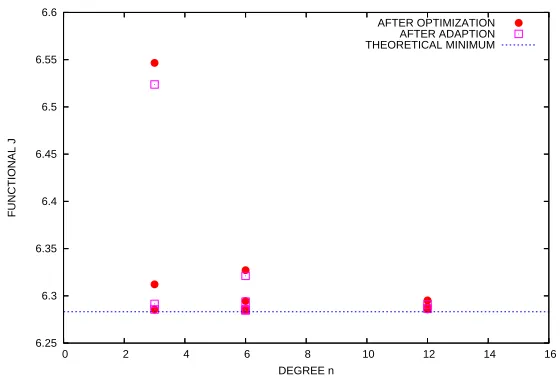
theorical minimum value is 2Π. The arc is successively parameterized by B´ezier curves of increasing degrees. The cost function values obtained with respect to the degree are depicted in figure (3).
6.25 6.3 6.35 6.4 6.45 6.5 6.55 6.6
0 2 4 6 8 10 12 14 16
FUNCTIONAL J
DEGREE n
COUPLING OPTIMIZATION WITH ADAPTION
AFTER OPTIMIZATION AFTER ADAPTION THEORETICAL MINIMUM
Figure 3. Results for the model problem : cost function values obtained after a single
opti-mization and then after adaption+optiopti-mization, for different parameterization degrees.
2.2.
Aerodynamic shape optimization
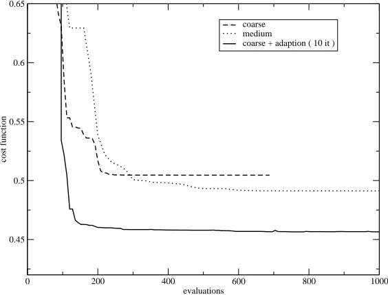
The proposed method is now faced with the aerodynamic optimization of the shape of a wing of a business aircraft [1] (courtesy of Piaggio Aero Ind.). The compressible flow is modeled by the Euler equations, which are solved using a finite-volume approach on unstructured meshes. The shape deformation is parameterized using the FFD approach described above. Figure (1) shows the wing shape embedded in the FFD lattice. The optimization procedure relies on the Multi-directional Search Algorithm (MSA) from Torczon [7], which is a derivative-free method similar to the well-known Nelder-Mead simplex method, but designed for parallel computations. The aim of the optimization is the reduction of the drag, including a constraint on the lift.
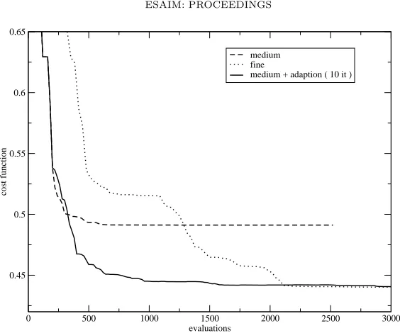
Optimization exercises are carried out using a coarse parameterization (8 d.o.f.), a medium one (20 d.o.f.) and a fine one (32 d.o.f.), with and without adaption. For the tests with adaption, the parameterization adaption procedure is performed every ten iterations, yielding a regular parameterization update until convergence of both optimization and adaption procedures. This strategy promotes the avoiding of local minima. Figure (4) shows the evolution of the cost function using a coarse parameterization with and without adaption and a medium parameterization without adaption. As can be observed, the use of the adaption procedure yields a faster convergence towards a shape of better fitness. Finally, the use of a coarse but adapted parameterization is more effective than the use of a medium but na¨ıve one. The results obtained using a medium parameterization (figure (5)) exhibit the same behavior. The optimum shapes found using the initial parameterization and the adapted parameterization are depicted in figure (6). As can be observed, the fitness improvement thanks to adaption corresponds to very slight modifications of the shape.
0 200 400 600 800 1000
evaluations 0.45
0.5 0.55 0.6 0.65
cost function
coarse medium
coarse + adaption ( 10 it )
Figure 4. Evolution of the cost function with and without adaption using a coarse parameterization.
3.
Conclusion
A self-adaptive parameterization methodology for shape optimization has been developed. It relies on the regularization of the design variables subject to the constraint that the shape remains unaltered in a least-squares sense. Its efficiency has been demonstrated for a geometrical model problem using B´ezier curves, and then for the aerodynamic shape optimization of a wing using the FFD approach.
0 500 1000 1500 2000 2500 3000 evaluations
0.45 0.5 0.55 0.6
cost function
fine
medium + adaption ( 10 it )
Figure 5. Evolution of the cost function with and without adaption using a medium parameterization.
0 1000 2000 3000
-400 -200 0 200 400
optimized shape optimized shape with adaption
Figure 6. Comparison of the shapes obtained (root and tip section).
References
[1] M. Andreoli, A. Janka, and J.-A. D´esid´eri. Free-form deformation parameterization for multilevel 3D shape optimization in aerodynamics. INRIA Research Report 5019, November 2003.
[2] J.-A. D´esid´eri. Two-level ideal algorithm for parametric shape optimization.Journal of Numerical Mathematics, 14, 2006. [3] J.-A. D´esid´eri, B. Abou El Majd, and A. Janka. Nested and self-adaptive b´ezier parameterization for shape optimization. In
International Conference on Control, Partial Differential Equations and Scientific Computing, Beijing, China, September 13-16 2004.
[4] J.-A. D´esid´eri and J.-P. Zol´esio. Inverse shape optimization problems and application to airfoils.Control and Cybernatics, 34(1), 2005.
[5] R. Duvigneau. Adaptive parameterization using free-form deformation for aerodynamic shape optimization. INRIA Research Report RR-5949, July 2006.