Introduction to diffuse interfaces and transformation fronts modelling in compressible media

C. Bourdarias, S. Gerbi, Editors

INTRODUCTION TO DIFFUSE INTERFACES AND TRANSFORMATION

FRONTS MODELLING IN COMPRESSIBLE MEDIA

Richard Saurel

and Fabien Petitpas

Abstract. Computation of interfaces separating compressible materials is related to mixture cells appearance. These mixture cells are consequences of fluid motion and artificial smearing of discon-tinuities. The correct computation of the entire flow field requires perfect fulfillment of the interface conditions. In the simplest situation of contact interfaces with perfect fluids, these conditions corre-spond to equal normal velocities and equal pressures. To compute compressible flows with interfaces two main classes of approaches are available. In the first one, the interface is considered as a sharp discontinuity. Lagrangian, Front Tracking and Level Set methods belong to this class. The second option consists in the building of a flow model valid everywhere, in pure materials and mixture cells, solved routinely with a unique Eulerian algorithm [37]. In this frame, the interface is considered as a numerically diffused zone, captured by the algorithm. There are some advantages with this approach, as the corresponding flow model is not only valid in artificial mixture cells, but it also describes accu-rately true multiphase mixtures of materials.

The [37] approach has been simplified by [22] with the help of asymptotic analysis, resulting in a sin-gle velocity, sinsin-gle pressure but multi-temperature flow model. This reduced model presents however difficulties for its numerical resolution as one of the equations is non-conservative. In the presence of shocks, jump conditions have been provided by [42], determined in the weak shock limit. When compared against experiments for both weak and strong shocks, excellent agreement was observed. These relations have been accepted as closure shock relations for the [22] model and allowed the study of detonation waves in heterogeneous energetic materials. Generalized Chapman-Jouguet conditions were obtained as well as heterogenous explosives (non-ideal) detonation wave structures [36].

Oppositely to the previous example of exothermic reactions and high speed flows, endothermic reac-tions are considered in [43] to deal with cavitating and flashing flows. In conjunction with capillary [33] and diffusive effects, it has been possible to deal with boiling flows [25].

Extra multiphysic extensions such as dynamic powder compaction [38], solid-fluid coupling in extreme deformations [12] have been investigated too.

1 _{Aix-Marseille Universit´e, CNRS, IUSTI UMR 7343, 5 rue E. Fermi, 13453, Marseille, France} 2 _{Also, RS2N, Bastidon de la Caou, 13360 Roquevaire, France}

c

EDP Sciences, SMAI 2013

R´esum´e. La r´esolution num´erique des probl`emes `a interfaces entre milieux compressibles est forte-ment li´ee `a l’apparition de ’mailles de m´elange’. Celles-ci sont li´ees au mouvement des fluides sur mail-lages fixes, induisant une diffusion artificielle des discontinuit´es de contact. La r´esolution num´erique de l’ensemble de l’´ecoulement n´ecessite le respect des conditions d’interface, qui correspondent pour les fluides parfaits `a l’´egalit´e des vitesses normales et `a l’´egalit´e des pressions.

Pour r´esoudre les ´ecoulements de fluides compressibles en pr´esence d’interfaces mat´erielles, essen-tiellement deux cat´egories de m´ethodes sont disponibles. Dans la premi`ere cat´egorie, l’interface est consid´er´ee comme une discontinuit´e. Les m´ethodes lagrangiennes, de ’suivi de front’ et Level Set ap-partiennent `a cette cat´egorie. La seconde option consiste en la construction d’un mod`ele d’´ecoulement valide partout, dans les milieux purs ainsi que dans les zones de m´elange, r´esolu routini`erement avec un unique solveur eul´erien [37]. Dans ce contexte, les interfaces sont trait´ees en tant que zones de diffusion num´erique, captur´ees par l’algorithme. Cette approche pr´esente certains avantages. Par exemple, le mod`ele d’´ecoulement n’est pas seulement valable dans les mailles de m´elange artificiel, mais aussi dans les zones d’´ecoulement diphasiques d’origine physique et ayant des ´evolutions hors d’´equilibre. L’approche de [37] a ´et´e simplifi´ee par [22] sur la base d’une analyse asymptotique dans la limite de forts coefficients de relaxation des vitesses et des pressions. Cette analyse conduit `a un mod`ele `a une seule vitesse et une seule pression, mais en d´es´equilibre de temp´eratures. La r´esolution num´erique de ce mod`ele pr´esente n´eanmoins certaines difficult´es, en raison du caract`ere non conservatif d’une des ´equations. En pr´esence d’ondes de choc, des relations de saut ont ´et´e propos´ees [42] et justifi´ees dans la limite des chocs faibles. Ces relations ont ´et´e valid´ees par rapport `a toutes les exp´eriences disponibles, `

a la fois pour les chocs faibles et forts. Elles ont donc ´et´e accept´ees comme relations de fermeture aux chocs pour le mod`ele de [22] et ont permis l’´etude des ondes de d´etonation dans les mat´eriaux ´energ´etiques h´et´erog`enes. Des conditions de Chapman-Jouguet g´en´eralis´ees ont ´et´e obtenues ainsi que la structure des ondes de d´etonation correspondantes (non id´eales) [36].

A l’oppos´e des situations pr´ec´edentes de transformations exothermiques dans des ´ecoulements `a grandes vitesses, des r´eactions d’´evaporation endothermiques ont ´et´e consid´er´ees [43] pour traiter les ´ecoulements cavitants et l’´evaporation ’flash’. Lorsque cette mod´elisation de la transition de phase est combin´ee aux effets capillaires [33] et diffusifs, il est possible de traiter la simulation num´erique directe de l’´ebullition nucl´e´ee [25].

Enfin, d’autres extensions sont aussi envisageables, telles que la compaction dynamique des poudres [38] ou le couplage solide-fluide en d´eformations extrˆemes [12].

Introduction

The computation of interfaces and waves dynamics with compressible materials has many fundamental and industrial applications, ranging from fluid mechanics and astrophysics to chemical, mechanical and environ-mental engineering. When dealing with compressible materials the main issue is related to the appearance of mixture cells. These mixture cells are consequences of fluid motion and artificial smearing of discontinuities. The correct computation of the entire flow field requires perfect fulfillment of the interface conditions. In the simplest situation of contact interfaces with perfect fluids, these conditions correspond to equal normal veloc-ities and equal pressures. To compute compressible flows with interfaces two main classes of approaches are available. In the first one, the interface is considered as a sharp discontinuity. To avoid as far as possible interface numerical smearing several options are possible:

• Lagrangian and ALE methods (see for example [11, 19]). In this context, the computational mesh moves and distorts with the material interface. However, when dealing with fluid flows, deformations are unbounded and resulting mesh distortions may result in computational failure [45].

by the volume fraction, transported by the flow. This method is widely used for incompressible flows as there is no thermodynamics to compute in mixture cells [17]. For compressible flows, extra energy equations are used as well as pressure relaxation procedures [4,29]. Multiphase flow ingredients are used with these methods that come quite close to the diffuse interface methods discussed later.

• Level-Set methods [30, 31, 47] are very popular methods to spatially locate interfaces. Special manage-ment of the interfaces is needed to preserve jump conditions. Relevant work in this direction was done by [13] with the Ghost Fluid Method.

• Front Tracking methods consider explicit interface tracking over a fixed Eulerian mesh [15, 27].

With the various preceding methods, the interface is managed with a specific treatment, having consequences with respect to coding complexity, conservation issues, extra physics extension capabilities and robustness especially in severe conditions. The second class of approaches follows another philosophy, closer to the one of capturing methods. Capturing methods are fundamental contributions of [52] and [16]. The aim was to solve the same equations with the same numerical scheme in both smooth and discontinuous flow regions. Pioneer works in ?’interface capturing’ or ?’diffuse interfaces’ modelling areas were done about forty years latter by [23]. Indeed, interfaces computation posed extra difficulties linked to thermodynamic state computation in artificial mixture zones. Determination of thermodynamic flow variables in these mixture zones has been achieved on the basis of multiphase flow modelling by [37]. Some advantages appeared:

• As already mentioned, the same equations are solved everywhere (interfaces, shocks, expansions waves) with a unique flow solver.

• These models and methods are able to dynamically create interfaces (not present initially) as for example in cavitating flows [41, 43].

• These methods are also able to deal with interfaces separating pure fluids and fluid mixtures, as for example when a granular material is in contact with a fluid [9, 38].

• As this approach includes the two velocities flow model of [2] it is also possible to compute velocity non-equilibrium bubbly or granular flows in conjunction with material interfaces [14, 39].

In the same period of time, a reduced model has been built by [22]. Here, pressure and velocity equilibrium is assumed, rendering the resulting model unable to deal with velocity non-equilibrium mixtures, but resulting in a more appropriate model for interface computations.

As it is more convenient to add extra physics in a single velocity context, multiphysics capabilities have been considered in the [22] framework. Surface tension modelling [33], shock and detonation computation in het-erogeneous materials [36, 42], phase transition [43], elastic solid - fluid coupling [12], powder compaction [38], interpenetration effects at unstable interfaces [40] are examples of such extensions.

To summarize, diffuse interface modelling allows quite advanced multiphysics extensions still solving a unique set of hyperbolic partial differential equations with a unique Godunov type flow solver.

1.

_{Total disequilibrium mixtures}

The [22] model we are going to use for the various multiphysics extensions comes from a more general model, out of mechanical, thermal and chemical equilibrium. The non-equilibrium mixture model presented hereafter consists in a symmetric formulation of the [2] model developed in [39]:

                  

                 

∂α1 ∂t +uI

∂α1

∂x =µ(p1−p2),

∂α1ρ1 ∂t +

∂α1ρ1u1 ∂x = 0,

∂α1ρ1u1 ∂t +

∂α1ρ1u21+α1p1 ∂x =pI

∂α1

∂x −λ(u1−u2)

∂α1ρ1E1 ∂t +

∂α1(ρ1E1+p1)u1 ∂x

=pIuI

∂α1 ∂x −λu

′

I(u1−u2)−p′_Iµ(p1−p2)

(1)

The second phase obeys a symmetrical set of equations.

Notations are conventional: αk, ρk, uk, pk represent respectively the volume fraction, the density, the velocity and the pressure of phase k. The total energy of phase k is defined byEk =ek+ 1/2u2k, withek the internal energy of phase k. This model is hyperbolic and fulfills the second law of thermodynamics. The closure relations for the relaxation parameters (µ andλ ) as well as for interfacial variables estimatesuI, u′I, pI, p′I are given in the same reference. This model is able to describe two-phase mixtures out of velocity equilibrium. Waves propagation is preserved thanks to the hyperbolic character of the equations and to the presence of relaxation effects. This model can be used for the computation of interface problems with perfect fulfillment of interface conditions. This goal can be reached with two different options:

• The first option consists in using stiff mechanical relaxation parametersµandλ[37].

• The second one is based on non-conservative termsuI

∂α1 ∂x andpI

∂α1 ∂x [1].

The first method is simple and robust. The second one is more subtle but renders possible the consideration of zones out of velocity equilibrium in conjunction with macroscopic interfaces where normal velocities and pressures have to be equal. In particular, it is able to deal with bubbles clouds crossing through material interfaces.

Consideration of extra physics is this formulation is possible but easier in the framework of single velocity formulations. The rest of this paper places in this context, as single velocity models are suitable for many applications.

2.

_{Mechanical equilibrium model, diffuse interfaces}

the non-equilibrium model and stiff mechanical relaxation. It reads:

                     

                    

∂α1 ∂t +u

∂α1

∂x =α1α2 ρc2

w

ρ1c21ρ2c22

ρ2c22−ρ1c21 ∂u

∂x,

∂α1ρ1 ∂t +

∂α1ρ1u ∂x = 0,

∂α2ρ2 ∂t +

∂α2ρ2u ∂x = 0,

∂ρu ∂t +

∂ρu2_+p ∂x = 0

∂ρE ∂t +

∂(ρE+p)u ∂x = 0

(2)

The total energy is defined as E =Y1e1+Y2e2+ 1/2u2 where Yk = (αkρk)/ρ represent the mass fraction of phasekandρ=α1ρ1+α2ρ2 the mixture density. This model is hyperbolic too with the same wave speeds as the gas dynamic equations but with the [53] sound speed, that presents a non monotonic behaviour with respect to the volume fraction: 1/ ρc2

w

=α1/ ρ1c21

+α2/ ρ2c22

. The equation of state allowing the thermodynamic closure is obtained from the mixture energy definition and the pressure equilibrium condition. This equation of state involves at least three arguments: p=p(ρ, e, α1) . For example, when each phase obeys the stiffened gas equation of state (see [26] for parameters determination),

pk= (γk−1)ρkek−γkp∞,k (3)

The mixture equation of state then reads:

p(ρ, e, α1, α2) = ρe−

_α 1γ1p∞,1 γ1−1

+α2γ2p∞,2 γ2−1

α1 γ1−1

+ α2

γ2−1

(4)

Parametersγk andp∞,kare characteristic constants of materialk. As this model involves a single pressure but two mass equations and a volume fraction equation, it is possible to determine two temperatures (Tk =Tk(p, ρk)) and two entropies. This feature is useful for phase transition modelling.

This model is an excellent candidate for interface problem computations. However, two difficulties at least are present:

• Rankine-Hugoniot relations cannot be determined in a conventional way as the volume fraction equation is non-conservative. With other sets of variables (entropy for example), it is no more possible to obtain meaningful jump conditions.

• The numerical resolution of this model is intricate, due to the presence of the same equation.

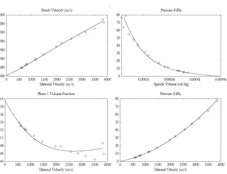
Figure 1. Comparison between experiments (symbols) and results obtained from Rankine-Hugoniot relations (5) for the Epoxy-Spinel mixture. Excellent agreement is observed. The same agreement is observed for all mixtures free of phase transition having experimental data in the Russian and American databases.

and American databases have been used in this aim. The corresponding algebraic system reads:

[αkρk(u−σ)] = 0, fork= 1,2

[ρu(u−σ) +p] = 0

ek−e0k+

p+p0 2 (vk−v

0

k) = 0, fork= 1,2 withvk= 1/ρk

(5)

3.

_{Simple and efficient relaxation method}

To solve System (2), an extended system is considered, that seems more complex at a first glance. However, with this extended system, there is no difficulty to preserve volume fraction positivity. Also, the sound speed with the new model is monotonic with respect to the volume fraction. Last, the Riemann problem resolution is straightforward as will be shown later, as the volume fraction is constant across the right and left facing waves. Nevertheless, to recover solutions of the mechanical equilibrium model (2), stiff pressure relaxation has to be used, preserving volume fraction positivity too. Therefore, the model is solved in a sequence of three steps:

• Solve the extended pressure non-equilibrium flow model, in the abscence of relaxation terms, with appropriate hyperbolic solver.

• Relax the pressure toward mechanical equilibrium and determine the volume fraction at pressure equi-librium.

• Compute the pressure with the mixture equation of state (4) based on the relaxed volume fraction and total energy, that results of the additional conservation law (7). Then reset the internal energies with the help of the mixture pressure, phases densities and appropriate equations of state.

Each step is summarized hereafter. The pressure non-equilibrium model reads:

                                                   ∂α1 ∂t +u

∂α1

∂x =µ(p1−p2),

∂α1ρ1 ∂t +

∂α1ρ1u ∂x = 0,

∂α2ρ2 ∂t +

∂α2ρ2u ∂x = 0,

∂ρu ∂t +

∂ρu2_+α

1p1+α2p2

∂x = 0

∂α1ρ1e1 ∂t +

∂α1ρ1e1u ∂x +α1p1

∂u

∂x =−pIµ(p1−p2),

∂α2ρ2e2 ∂t +

∂α2ρ2e2u ∂x +α2p2

∂u

∂x =pIµ(p1−p2)

(6)

This system can be easily derived from System (1) in the limit of stiff velocity relaxation.

With System (6) combination of the internal energy equations with mass and momentum equations results in the additional mixture energy equation:

∂ρ

Y1e1+Y2e2+ 1 2u 2 ∂t + ∂ ρ

Y1e1+Y2e2+ 1 2u

2

+ (α1p1+α2p2)

u

∂x = 0 (7)

This extra equation is important during numerical resolution, in order to correct inaccuracies due to the nu-merical approximation of the non-conservative internal energy equations in the presence of shocks.

This model exhibits a nice feature regarding the mixture sound speed that reads,

c2f =Y1c21+Y2c22

and has a monotonic behaviour versus volume and mass fractions. It represents the frozen mixture speed of sound with respect to the pressure relaxation effects. The model is thus hyperbolic with waves speeds: u+cf ,

System (6) is aimed to replace direct resolution of System (2) by the three steps method mentioned previously. During the first step, System (6) is solved in absence of relaxation terms (µ= 0). Then relaxation terms are considered and are assumed stiff. In other word, the mechanical equilibrium solution is obtained at the end of the second step. It can be proved by asymptotic analysis that such strategy yields precisely to System (2) (see [44] Appendix B for the details).

Numerical resolution of the pressure non-equilibrium model in the limit of stiff pressure relaxation is then addressed. In regular zones, this model is self consistent. But in the presence of shocks the internal energy equations are inappropriate. To correct the thermodynamic state predicted by these equations in the presence of shocks, the total mixture energy equation is used. This correction is valid on both sides of the interface, when the flow tends to the single phase limit. The details of this correction will be examined further. For now, the pressure non-equilibrium system (6) is augmented by the redundant equation (7).

3.1.

Hyperbolic solver

The hyperbolic solver is aimed to solve System (6-7) in the absence of relaxation terms (µ= 0). The first ingredient corresponds to the Riemann solver used to compute the fluxes that cross each cell boundary. Then the variables are updated with a Godunov type method.

3.1.1. HLLC Riemann solver

The [51] solver is considered at cell boundaries, separating left (L) and right (R) states. This solver involves 3 waves, is genuinely positive and valid for any convex equation of state. It is thus an excellent candidate for the various applications we are dealing with. The left- and right-facing waves speeds are readily obtained, following [10] estimates,

SR= max (uL+cL, uR+cR), SL= min (uL−cL, uR−cR),

where the sound speed still obeys the frozen sound speed relation,c2

R,L=Y1R,Lc21R,L+Y2R,Lc22R,L. The intermediate wave speed is estimated under HLL approximation,

SM =

ρu2_+p

L− ρu 2_+p

R−SL(ρu)L+SR(ρu)R (ρu)L−(ρu)R−SLρL+SRρR

,

with the mixture density and mixture pressure defined previously. From these wave speeds, the following variable states are determined,

(αkρk) ∗

R= (αkρk)R

SR−uR

SR−SM

, (αkρk) ∗

L= (αkρk)L

SL−uL

SL−SM

,

p∗

=pR+ρRuR(uR−SR)−ρ∗RSM(SM−SR), withρ∗

R,L= (α1ρ1) ∗

R,L+ (α2ρ2) ∗ R,Land,

E∗ R=

ρRER(uR−SR) +pRuR−p∗SM

ρ∗

R(SM −SR)

, E∗ L=

ρLEL(uL−SL) +pLuL−p∗SM

ρ∗

L(SM −SL)

,

withE=Y1e1+Y2e2+ 1 2u

2_{. The upperscript ’*’ stands for the Riemann problem solution states.}

The volume fraction jump is readily obtained, as in the absence of relaxation effects the volume fraction is constant along fluid trajectories,

αk ∗

R=αkR, αk ∗

L=αkL.

As the volume fraction is constant across left- and right-facing waves, the fluid density is determined from the preceding relations:

ρ∗

kR,L=ρkR,L

uR,L−SR,L

Internal energy jumps are determined with the help of approximate Hugoniot relations for System (6). Let us consider the example of fluids governed by the stiffened gas EOS (3). With the help of the EOS, the phasic pressures are constrained along their Hugoniot curves as functions only of the corresponding phase density,

p∗ kR,L(ρ

∗

kR,L) = pkR,L+p∞k

(γk−1)ρkR,L−(γk+ 1)ρ∗kR,L (γk−1)ρ∗kR,L−(γk+ 1)ρkR,L

−p∞k

The phases internal energies are then determined from the EOS: e∗ kR,L=e

∗ kR,L(p

∗ kR,L, ρ

∗ kR,L) . Equipped with this solver, the next step is to develop a Godunov type scheme.

3.1.2. Godunov type method

In the absence of relaxation terms, the conservative part of System (6) is updated with the conventional Godunov scheme:

Un+1

i =U

n i −

∆t

∆x F

∗

(Uin, Uin+1)−F ∗

(Uin−1, U n i )

with U = ((αρ)_k, ρu, ρE)T and F = ((αρ)_ku, (ρu+ (α1p1+α2p2)), (ρE+ (α1p1+α2p2))u)T. The volume fraction equation is updated with the Godunov method for advection equations:

αkni+1=αkni − ∆t

∆x

(uαk)∗i+1/2−(uαk)∗i−1/2−αkni,l(u ∗

i+1/2−u ∗ i−1/2)

This scheme guarantees volume fraction positivity during the hyperbolic step. Obviously, higher order extension of the Godunov method can be considered.

Regarding the non-conservative energy equations, there is no hope to determine accurate numerical approxima-tion in the presence of shocks [21]. Therefore, we use the simplest approximaapproxima-tion of the corresponding equaapproxima-tions by assuming the product (αp)_k,n

i constant during the time step:

(αρe)_kn_,i+1= (αρe)_k,n_i − ∆t ∆x

(αρeu)_k,∗

i+1/2−(αρeu)k ∗

,i−1/2+ (αp)k, n i

u∗

i+1/2−u ∗ i−1/2

The lack of accuracy in the internal energy computation resulting from the present scheme is not so crucial. The internal energies will be used only to estimate the phases pressures at the end of the hyperbolic step, before the relaxation one. The relaxation step will give a first correction to the internal energies, in agreement with the second law of thermodynamics. A second correction will be made with the help of the total mixture energy. The details of these two steps are described in the next subsections.

3.2.

Relaxation step

equilibrium model (2). In the relaxation step the system to consider reads,                                                                ∂α1

∂t =µ(p1−p2),

∂α1ρ1 ∂t = 0,

∂α2ρ2 ∂t = 0,

∂ρu ∂t = 0

∂α1ρ1e1

∂t =−pIµ(p1−p2),

∂α2ρ2e2

∂t =pIµ(p1−p2),

∂ρE ∂t = 0

(8)

in the limitµ→+∞.

After some manipulations the internal energy equations become:

∂e_k ∂t +pI

∂v_k ∂t = 0

This system can be written in integral form as,

ek−e0k+ ˆpIk(vk−vk0) = 0

with ˆp_Ik= 1 vk−v

0 k

∆t

R

0

pI∂v_∂tkdt.

Determination of pressure averages has to be done in agreement with thermodynamic considerations. By summing the internal energy equations we have:

X

k

Ykek−Yke0k

+X

k ˆ

pIk(Ykvk−Ykvk0) = 0

As the system conserves energy,P

k

Ykek−Yke0k

= 0.

On the other hand, mass conservation implies,P

k

(Ykvk−Ykvk0) = 0.

Therefore, the identity,

X

k

Ykek−Yke0k

+X

k ˆ

p_Ik(Ykvk−Ykvk0) = 0

is fulfilled if the various pressure averages are taken equal, i.e.,

ˆ

This pressure average estimate also agrees with the entropy inequality. The system to solve is thus composed of equations,

ek(p, vk)−e0k(p0k, vk0) + ˆpI(vk−vk0) = 0, fork= 1,2 (9)

which involves 2+1 unknowns, vk(k= 1,2) andp. Its closure is achieved by the saturation constraint,

X

k

αk= 1,

that is rewritten under the form,

X

k

(αρ)_kvk(p) = 1. (10)

As the (αρ)_k are constant during the relaxation process, this system is replaced by a single equation with a single unknown (p). With the help of the EOS (3) the energy equations (9) become,

vk(p) =v0k

p0

k+γkp∞k+ (γk−1)ˆpI

p+γkp∞k+ (γk−1)ˆpI

and thus the only equation to solve (for p) is (10).

Once the relaxed pressure is found, the phases specific volumes and volume fractions are determined. However, there is no guarantee that the mixture EOS or the mixture energy be in agreement with this relaxed pressure. In order to respect total energy and correct shock dynamics on both sides of the interface, the following correction is employed.

3.3.

Reset step

As the volume fractions have been estimated previously by the relaxation method, the mixture pressure can be determined from the mixture EOS based on the mixture energy which is known from the solution of the total energy equation. As the mixture total energy obeys a conservation law, its evolution is accurate in the entire flow field and in particular at shocks.

Again considering fluids governed by the stiffened gas EOS, the mixture EOS is given by (4). This EOS is valid in pure fluids and in the diffuse interface zone. As it is valid in pure fluids and based on the total energy equation, it guarantees correct wave dynamics on both sides of the interface. Inside the numerical diffusion zone of the interface, numerical experiments show that the method is accurate too, as the volume fractions used in the mixture EOS have a quite accurate prediction from the relaxation step.

To summarise, the pressure at the end of the time step is computed with the mixture EOS (4) as:

pn+1_=p(ρn+1_{, e}n+1_{, α}relax

k ), (11)

whereρn+1_anden+1_{represent respectively the mixture density and mixture internal energy at timet}n+1_{, while} αrelax

k represent the volume fractions determined at the end of the relaxation step. Once the mixture pressure is determined the internal energies of the phases are reset with the help of their respective EOS before going to the next time step,

en_k+1=ek(pn+1, αkρkn+1, αkn+1), (12)

3.4.

Shock propagation in multiphase mixture

When the flow involves material interfaces only, the preceding algorithm is particularly simple and efficient. But in some situations, physical mixtures of materials are under interest, eventually in the presence of shocks. This occurs for example in the study of shocks and detonation waves in heterogeneous materials. In this situation, the shock energy has to be apportioned correctly among the phases; otherwise the shock speeds as well as the various jumps are incorrect. The goal is thus to impose the shock conditions (5) in the pressure equilibrium solution. This issue has been addressed in [34] and a solution method was given in [36]. It consists in replacing Equations (9) in the previous pressure relaxation step by,

ek(p, vk)−ek0(p0k, v0k) +

p+p0 2 (vk−v

0

k) = 0, fork= 1,2 (13)

where the state with superscript 0 indicates the Hugoniot pole. This state has to be constant inside the shock layer. To do this, additional evolution equations are used to replace the internal energy equations of System (6), in the shock layer only. These equations read:

    

   

∂v0 k

∂t +u ∂v0

k

∂x = 0, fork= 1,2

∂p0 ∂t +u

∂p0 ∂x = 0

(14)

Thanks to (13) and (14) the method converges to the correct shock state.

3.5.

Summary of the numerical method

The numerical method can be summarized as follows:

• At each cell boundary, solve the Riemann problem of System (6) in the absence of relaxation terms with the HLLC solver or any positive Riemann solver.

• Evolve all flow variables with the Godunov method or higher order extensions.

• Determine the relaxed pressure and especially the volume fraction by solving Equation (10) with the help of the Newton method. Equations (9) are used if interfaces separate pure fluids. If one of the media corresponds to a multiphase mixture, Equations (9) are replaced by (13). In this instance, (14) have to be solved in the shock layer. The shock layer is detected thanks to shock indicators such as [50] (see paragraph 14.6.4) or [28].

• Compute the mixture pressure with Equation (4).

• Reset the internal energies with the computed pressure with the help of their respective EOS (12). • Go to the first item for the next time step.

3.6.

Computational example

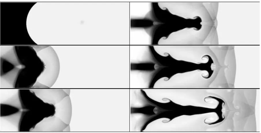
A non-conventional computational example is shown in the Figure 2. A piston impacts a liquid column with a curved liquid-gas interface. A Richtmyer-Meshkov type instability appears, as expected. Unexpected features appear too, as cavitation pockets are created in the liquid domain, due to liquid jet presence. To deal with such a flow, the model has to deal with material interfaces, shocks and expansions waves. It must also predict dynamic interfaces appearance. Cavitation pockets are here consequences of the small amount of gas present in the liquid that grows under expansion effects as a result of the pressure equilibrium condition.

Figure 2. Richmyer-Meshkov instability with a cavitating liquid and a non miscible gas.

4.

_{Capillary effects}

The following capillary flow model is a slight variation of the [33] model where the CSF method of [5] was embedded in the compressible Kapila model. The corresponding system reads:

                                                                 ∂α1

∂t +~u·∇~α1−

(ρ2c 2 2−ρ1c

2 1) ρ1c21

α1 +ρ2c

2 2 α2

div(~u) = 0, fork= 1,2

∂ρY1

∂t +div(ρY1~u) = 0

∂ρ

∂t +div(ρ~u) = 0

∂ρ ~u ∂t +div



P I+ρ ~u⊗~u−σ 

 ∇~Y1

I−

~

∇Y1⊗∇~Y1 ∇~Y1

  

=~0

∂ρ 

e+

σ ∇~Y1

ρ +

1 2k~uk

2 



∂t +div

   ρ  e+ σ ∇~Y1

ρ +

1 2k~uk

2 

+P 

~u−σ 

 ∇~Y1

I−

~

∇Y1⊗∇~Y1 ∇~Y1



.−→u 

= 0

(15)

Whereσrepresents the surface tension coefficient. This formulation presents at least two advantages:

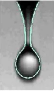
Figure 3. Comparison of computed drop formation under gravity effects (light lines) versus experimental photograph (grey contours). System (15) is solved everywhere, in pure liquid, pure gas and at the interface.

• There is no interface width, compared to the [6] second gradient theory that needs too fine resolution for practical applications.

A computation example and comparison with experiments is shown in the Figure 3. At the discrete level, when capillary effects are considered, care has to be done with the following specific points:

• The pressure is no longer constant at the contact discontinuity. The local interface curvature and surface tension effects are accounted for in the Riemann solver. Details are given in [33].

• Capillary effects cannot be activated with initial discontinuities in the mass fractions. Thus, the first computational time steps (less than 10) are acheived without surface tension, in order that artificial smearing render discrete mass fraction gradients available.

5.

_{Phase transition}

This extension has been done in [43] on the basis of entropy production examination. In the absence of capillary effects, the resulting system reads,

                                                   ∂α1

∂t +~u·∇~(α1) =

(ρ2c22−ρ1c21) ρ1c

2 1 α1

+ρ2c 2 2 α2

div(~u) +ρν(g2−g1) c2 1 α1 + c 2 2 α2 ρ1c

2 1 α1

+ρ2c 2 2 α2

+H(T2−T1) Γ1 α1

+Γ2 α2 ρ1c

2 1 α1

+ρ2c 2 2 α2

∂α1ρ1

∂t +div(α1ρ1~u) =ρν(g2−g1)

∂α2ρ2

∂t +div(α2ρ2~u) =−ρν(g2−g1)

∂ρ~u

∂t +div(ρ~u⊗~u) +∇~(p) = 0

∂ρE

∂t +div((ρE+p)~u) = 0

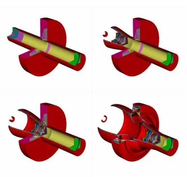
Figure 4. Cavitating flow around a hypervelocity underwater missile. Combustion gases are shown in yellow contours and are in contact with vapour, in blue colour. The vapour is separated from the liquid (not shown) by an evaporating interface. Two different types of interfaces are thus present in this example. The results are issued from [35].

with the following notations: gk =hk−Tksk represents the Gibbs free energy,H represents the temperature relaxation parameter andν the mass transfer kinetics.

Some comments are due regarding the volume fraction equation. The first term in the right hand side, present in the [22] model, represents mechanical relaxation effects, present in all zones where the velocity divergence is non zero (shocks, compressions, expansions). The second term represents volume variations due to mass transfer, in a context where both phases are compressible. The last group of terms represents dilatation effects due to heat transfer. Γk represents the Gruneisen coefficient of the phase k.

The model needs thermodynamic parameters on one hand and kinetics ones, such as H and ν on the other hand. In the present formulation, each fluid has its own thermodynamics and the equation of state parameters are determined on the basis of the phase diagram, as detailed in [26]. Regarding kinetic parameters, we have learnt in the beginning of this paper that it was possible to fulfill interface conditions of simple contact by using infinite mechanical relaxation parameters. Here, infinite thermal and mass transfer kinetics are used (infinite H andν). It means that local thermodynamic equilibrium is assumed. This renders possible the consideration of phase transition fronts propagating at global finite rate [43]. It is shown in this reference that phase transition fronts propagate in metastable liquids at the characteristic speed of the full equilibrium system. This is indeed the system that is solved at the evaporating interface. It consists in the mixture mass, momentum and energy equations, closed by pressure, temperature and Gibbs free energy equilibrium conditions. The associated sound speed is very low and the lower CJ point conditions [7, 8, 48, 49] merge with the aforementioned characteristic speeds.

6.

_Detonations

To deal with the detonation of condensed energetic materials, possibly heterogeneous, the same flow model as previously can be used except regarding the equations of state that must contain appropriate reference energy yielding exothermic heat of reaction. For example, the stiffened gas equation of state (3) now expresses as,

pk= (γk−1)ρk(ek−qk)−γkp∞k

whereqk represents the reference energy.

It is then necessary to use finite rate heat and mass transfer coefficients, respectively H and ν. Let us present first an illustrative example. A detonation tube is filled with a heterogeneous explosive mixture. A shock wave is emitted by a detonator and transforms to a detonation that propagates in the explosive, loaded with aluminium particles.

Material interfaces are present too as 7 different materials have to be considered. As previously mentioned, the same equations are solved everywhere with the same flow solver. The results shown in the Figure 5 are taken from [36]. Starting from the flow model expressed in Section 5, it is possible to determine generalized Chapman Jouguet relations, yielding non-ideal detonation behaviour even in pure 1D plannar flow configuration. Indeed, expressing the flow model between the shock front and the sonic surface, in the detonation wave frame of reference, the following expression for the velocity divergence is obtained:

du¯

dx =

1

ρ(c2_−u¯2₎        Γ1 α1 Γ2 α2 ρ2c22

Γ2 −ρ1c

2 1 Γ1

ρ1c21

α1 +ρ2c

2 2 α2

H(T2−T1)

+      

ρ2c22 Γ2

−ρ1c 2 1 Γ1    

ρ1c21 α1

+ρ2c 2 2 α2   c2 1 α1 + c 2 2 α2

+h2− c2

2 Γ2

−

h1− c2 1 Γ1     ˙ m1 α1 Γ1

+α2 Γ2       

The generalized Chapman Jouguet relation appears immediately. On the sonic surface characterized by,

¯

Figure 5. Mixture density contours at the initial time and at three successive times showing detonation dynamics and interfaces motion for the detonation tube problem.

necessarily,

Γ1 α1

Γ2 α2

ρ2c22

Γ2 −ρ1c

2 1 Γ1

_ρ 1c21 α1

+ρ2c 2 2 α2

H(T2−T1)

+



  

ρ2c22

Γ2 −ρ1c

2 1 Γ1

_ρ 1c21 α1

+ρ2c 2 2 α2

c2 1 α1

+ c 2 2 α2

+h2− c2

2 Γ2

−

h1− c2

1 Γ1



  

˙

m1

α1 Γ1

+α2 Γ2

= 0

in detonation velocity. The explanation comes from the fact that, in temperature non-equilibrium conditions the phases have unconstrained dilatation. Indeed, due to the fast phenomenon occurring in the reaction zone and due to the quite large particle sizes, thermal equilibrium assumed in conventional CJ and ZND models is not justified and yields to underestimated detonation speeds, as a consequence of constrained dilatation of the various substances.

The present flow model, CJ conditions and ZND structure have been recently investigated in details by [46] for the study of highly non-ideal ammonium nitrate explosives, showing in particular impressive comparison with experimental detonation records in a broad range of confinements and wide range of charge diameters.

Let’s now turn back to the issue of kinetic coefficients determination (H and ν). In drastic flow conditions occuring in detonations, it is not possible to determine by direct measurements such parameters. In [3], analysing detonation experiments based on explosive liquids loaded with particles of different sizes, from 0.1 to 100µmit appeared that heat exchanges are negligible (H=0). This is due to the short particle life time in the detonation reaction zone. In [46] an inverse method based on detonation front curvature is given, allowing accurate determination of the decomposition rate kineticsν. The method given in this reference is a 2D extension of the well known [54] streamline method for curved detonation waves, widely used to find decomposition kinetics of explosives.

7.

_Perspectives

Diffuse interface methods are now mature enough to deal with realistic and advanced applications. There are however many fundamental issues to address:

• The shock relations (5) have been demonstrated for weak shocks. They have been compared to experi-mental data for strong shocks (in the megabar range) showing excellent agreement too [42]. However, there is a lack of mathematical proof for strong shocks.

• The numerical method summarized in Section 3 and its variants [32] are very efficient for high speed flows. However, many applications deal with low Mach number flow conditions and there is a clear need for efficient algorithms at all Mach number for diffuse interface models. Efforts in this direction have been done by [24].

• Another numerical issue deals with long time evolutions, where interfaces become too smeared with up-wind scheme computations. There is thus a clear need to sharpen interfaces without losing conservation properties.

• There are also extra mathematical modelling issues when dealing with extra physics extensions, such as for example, hot spot modelling in shock to detonation transition in the area of combustion, solid fluid coupling [12] to make a bridge between fluid and solid mechanics, the direct numerical simulation of boiling flows in the area of energetics.

• Another important modelling issue is related to velocity drift effects restoration in diffuse interface formulations. Attempts in this direction have been done by [18], [38] and [40].

The first author is particular grateful to St´ephane Gerbi and Christian Bourdarias for their kind invitation at the AMIS 2012 conference in Chambery.

References

[1] R. Abgrall and R. Saurel. Discrete equations for physical and numerical compressible multiphase mixtures.Journal of Com-putational Physics, 186(2):361–396, 2003.

[2] M. Baer and J. Nunziato. A two-phase mixture theory for the deflagration-to-detonation transition (DDT) in reactive granular materials.Int. J. of Multiphase Flows, 12:861–889, 1986.

[4] D. Benson. Computational methods inLagrangian and Eulerian hydrocodes.Computer method in Applied Mechanics and Engineering, 99:235–394, 1992.

[5] J. Brackbill, D. Kothe, and C. Zemach. A continuum method for modelling surface tension.Journal of Computational Physics, 100:335–354, 1992.

[6] J. Cahn and J. Hilliard. Free energy of a nonuniform system i: Interfacial free energy.J. Chem. Physics, 28(2):258, 1958. [7] H. Chaves. Changes of phase and waves on depressurization of liquids with high specific heat.Mitt. Max-Planck-Institut f. Str

¨

omungsforschung, 77, 1984.

[8] H. Chaves. Phasenubergange und wellen bei der entspannung von fluiden hoher spezifischer warme.Mitt. Max-Planck-Institut f. Str¨omungsforschung, 77, 1984.

[9] A. Chinnayya, E. Daniel, and R. Saurel. Computation of detonation waves in heterogeneous energetic materials.Journal of Computational Physics, 196:490–538, 2004.

[10] S. F. Davis. Simplified second orderGodunov type methods.SIAM J. Sci. Comp., 9:445–473, 1988.

[11] C. Farhat and F. Roux. A method for finite element tearing and interconnecting and its parallel solution algorithm. Interna-tional Journal for Numerical methods in Engineering, 32:457–492, 1991.

[12] N. Favrie, S. Gavrilyuk, and R. Saurel. Solid-fluid diffuse interface model in cases of extreme deformations.Journal of Com-putational Physics, 228(16):6037–6077, 2009.

[13] R. Fedkiw, T. Aslam, B. Merriman, and S. Osher. A non oscillatory Eulerian approach to interfaces in multimaterial flows (TheGhostFluidMethod).Journal of Computational Physics, 152:457–492, 1999.

[14] S. Gavrilyuk and R. Saurel. A compressible multiphase flow model with microinertia. Journal of Computational Physics, 175:326–360, 2002.

[15] J. Glimm, J. Grove, X. Li, K. Shyue, Q. Zhang, and Y. Zeng. Three dimensional front tracking.SIAM J. Scientific Computing, 19:703–727, 1998.

[16] S. Godunov. A finite difference method for numerical computation of discontinuous solutions of the equations of fluid dynamics.

Math Sb., 47:357–393, 1959.

[17] D. Gueyffier, L. Li, A. Nadim, R. Scardovelli, and S. Zaleski. Volume-of-fluid interface tracking with smoothed surface stress methods for three-dimensional flows.Journal of Computational Physics, 152:423–456, 1999.

[18] H. Guillard and F. Duval. A darcy law for the drift velocity in a two-phase flow model.Journal of Computational Physics, 224:288–313, 2007.

[19] C. Hirt, A. Amsden, and J. Cook. An arbitrary Lagrangian Eulerian computing method for all flow speeds. Journal of Computational Physics, 14:227–253, 1974.

[20] C. Hirt and B. Nichols. Volume of fluid (vof) method for the dynamics of free boundaries.Journal of Computational Physics, 39:201–255, 1981.

[21] T. Hou and P. Le Floch. Why non-conservative schemes converge to the wrong solution: Error analysis.Math. Comp., 62:497– 530, 1994.

[22] A. Kapila, R. Menikoff, J. Bdzil, S. Son, and D. Stewart. Two-phase modeling of DDT in granular materials: Reduced equations.Physics of Fluids, 13:3002–3024, 2001.

[23] S. Karni. Multicomponent flow calculations by a consistent primitive algorithm.Journal of Computational Physics, 112:31–43, 1994.

[24] S. Le Martelot, B. Nkonga, and R. Saurel. Liquid and liquid-gas flows at all speeds: Reference solutions and numerical schemes.

Journal of Computational Physics, in revision, 2013.

[25] S. Le Martelot, R. Saurel, and B. Nkonga. Towards the direct numerical simulation of nucleate boiling flows. Progress in Energy and Combustion Science, in preparation, 2013.

[26] O. Le Metayer, J. Massoni, and R. Saurel. Elaborating equations of state of a liquid and its vapor for two-phase flow models.

Int. J. of Thermal Sciences, 43:265–276, 2004.

[27] R. Leveque and K. Shyue. Two-dimensional front tracking based on high resolution wave propagation methods.Journal of Computational Physics, 123(2):354–368, 1996.

[28] R. Menikoff and M. Shaw. Reactive burn models and ignition and growth concept.Los Alamos National Laboratory Report, LA-UR-10-01870, 2010.

[29] G. Miller and E. Puckett. A high-orderGodunov method for multiple condensed phases.Journal of Computational Physics, 128(1):134–164, 1996.

[30] W. Mulder, S. Osher, and J. Sethian. Computing interface motion: The compressibleRayleigh-Taylor andKelvin-Helmholtz instabilities.Journal of Computational Physics, 100:209, 1992.

[31] S. Osher and R. Fedkiw. Level set methods: An overview and some recent results.Journal of Computational Physics, 169:463– 502, 2001.

[32] M. Pelanti and K. Shyue. A mixture energy consistent 6-equation two-phase model for fluids with interfaces and cavitation phenomena.Conference Applied Math. In Savoie (AMIS 2012), 19-22 june 2012, Chambery, France, 2012.

[33] G. Perigaud and R. Saurel. A compressible flow model with capillary effects.J. Comp. Phys., 209:139–178, 2005.

[35] F. Petitpas, J. Massoni, R. Saurel, E. Lapebie, and L. Munier. Diffuse interface models for high speed cavitating underwater systems.Int. J. of Multiphase Flows, 35(8):747–759, 2009.

[36] F. Petitpas, R. Saurel, E. Franquet, and A. Chinnayya. Modelling detonation waves in condensed energetic materials: Multi-phaseCJconditions and multidimensional computations.Shock waves, 19(5):377–401, 2009.

[37] R. Saurel and R. Abgrall. A multiphaseGodunov method for compressible multifluid and multiphase flows.Journal of Com-putational Physics, 150:425–467, 1999.

[38] R. Saurel, N. Favrie, F. Petitpas, M. Lallemand, and S. Gavrilyuk. Modeling dynamic and irreversible powder compaction.

Journal of Fluid Mechanics, 664:348–396, 2010.

[39] R. Saurel, S. Gavrilyuk, and F. Renaud. A multiphase model with internal degrees of freedom: Application to shock-bubble interaction.Journal of Fluid Mechanics, 495:283–321, 2003.

[40] R. Saurel, G. Huber, G. Jourdan, E. Lapebie, and L. Munier. Modelling spherical explosions with turbulent mixing and post-combustion.Physics of Fluids, 24:115101–42, 2012.

[41] R. Saurel and O. Le Metayer. A multiphase model for compressible flows with interfaces, shocks, detonation waves and cavitation.Journal of Fluid Mechanics, 431:239–271, 2001.

[42] R. Saurel, O. Le Metayer, J. Massoni, and S. Gavrilyuk. Shock jump relations for multiphase mixtures with stiff mechanical relaxation.Shock Waves, 16:209–232, 2007.

[43] R. Saurel, F. Petitpas, and R. Abgrall. Modelling phase transition in metastable liquids: application to cavitating and flashing flows.Journal of Fluid Mechanics, 607:313–350, 2008.

[44] R. Saurel, F. Petitpas, and R. Berry. Simple and efficient relaxation methods for interfaces separating compressible fluids, cavitating flows and shocks in multiphase mixtures.Journal of Computational Physics, 228(5):1678–1712, 2009.

[45] D. Scheffer and J. Zukas. Practical aspects of numerical simulation of dynamic events: material interfaces. International Journal of Impact Engineering, 24(5-6):821–842, 2000.

[46] S. Schoch, N. Nikiforakis, B. Lee, and R. Saurel. Multi-phase simulation of ammonium nitrate emulsion detonation.Combustion and Flame, in press, 2013.

[47] J. Sethian. Evolution, implementation and application of level set and fast marching methods for advancing fronts.Journal of Computational Physics, 169:503–555, 2001.

[48] J. Simoes-Moreira and J. Shepherd. Evaporation waves in superheated dodecane.J. Fluid Mech., 382:63–86, 1999.

[49] P. Thompson, H. Chaves, G. Meier, Y. Kim, and H. Speckmann. Wave splitting in a fluid of large heat capacity. J. Fluid Mech., 185:385–414, 1987.

[50] E. Toro.Riemann solvers and numerical methods for fluid dynamics. Springer Verlag, Berlin, 1997.

[51] E. Toro, M. Spruce, and W. Speares. Restoration of the contact surface in the hll riemann solver.Shock waves, 4:25–34, 1994. [52] Von Neuman and R. Richtmyer. A method for the numerical calculation of hydrodynamic shocks.Journal of Applied Physics,

21:232–237, 1950.

[53] A. Wood. A textbook of sound.G. Bell and Sons LTD, London, 1930.