Original Article
Analysis of incomplete longitudinal binary responses with Bayesian method
Habibollah Esmaily1, Fatemeh Salmani2*, Mohammad Reza Meshkani3, Anoushirvan Kazemnejad4, Nasser Reza Arghami5
1
Department of Biostatistics, Health Sciences Research Center Mashhad University of Medical Sciences, Mashhad, Khorasan Razavi, Iran
2
Department of Biostatistics, School of Paramedical Sciences, Shahid Beheshti University of Medical Sciences, Tehran, Iran 3
Department of Statistics, School of Mathematics Sciences, Shahid Beheshti University, Tehran, Iran 4
Department of Biostatistics, Medical Sciences, Tarbiat Modares University, Tehran, Iran 5
Department of Statistics, School of Mathematics sciences, Ferdowsi University, Mashhad, Khorasan Razavi, Iran
ARTICLE INFO ABSTRACT
Available online at: http://jbe.tums.ac.ir
Longitudinal study plays an important role in the epidemiological, clinical, and social science studies. In these kinds of studies, every individual is observed frequently during a period of time. The statistical analysis of longitudinal presents special opportunities and challenges. The repeated outcomes for one individual tend to be correlated among themselves also one of the problems that we face in longitudinal studies is the missing data. These two issues are taken into account in this article. By using the logit link function, designed for longitudinal data, we introduce a mixed model, and then present the evaluation of variance components by Bayesian methods. The applied method exploits the non-conjugate priors. The conjugate priors, however, are easier to deal with. Finally, an application of the model in a clinical experiment is presented.
Key words: longitudinal, binary, logit, bayes, non-cojugate
Introduction1
In many studies, the response variable observed for an individual in several times. Longitudinal study is a kind of survey in which, an individual characteristic is studied over time (1) Recorded response may be quantitative or categorical especially binary. Longitudinal studies compare to cross-sectional studies, are more accurate (1), but there is a problem that sometimes various reasons cause missing observations in some unites.
* Corresponding Author: Fatemeh Salmani, Postal Address: Department of Biostatistics, Shahid Beheshti University of Medical Sciences, Tehran, Iran.
Email: [email protected]
Elimination of unites with missing data not only lead to sample size reduction but also result in devastate of costs and bias in the final analysis (2). There are several ways of solving these problems.
Graze et al. employed a method which later became known as GSK method (3). Koch et al. (4), Woolson and Clarke (5) extended the above method to binary data with missing responses. The mentioned model called “fixed effects” model. In some studies, treatments or factors may be random, thus, use of “fixed effects” model does not work in such situations.
This paper is based on the assumption that treatments or explanatory variables have a random effect. Longitudinal binary responses for data with missing values were investigated and J Biostat Epidemiol. 2015; 1(3-4): 100-104.
parameters were estimated using Bayesian method and compared with “restricted maximum likelihood” method.
Statistical Models for Longitudinal Studies with Binary Responses
Model employed by Kazemnejad and Meshkani (6) was the generalization of the GSK method. According to the little in this model, the missing data were missing completely at random (2).
A contingency table is formed from response categories and subgroups. They write the formed vectors as a column vector and call it observations vector. Hence, any single missing data would be taken into consideration. With the observations vector and matrix operations of values, will be calculated (6).
Logit (P) vector is called F (P), where P is a vector of success ratio which is made based on sub-groups of population and repetition times. Hence, F (P) is a function of P and P is a function of explanatory variables. With this assumption that the treatment factor is random and F (P) asymptotically follows the normal distribution, F (P) is considered as y, the following mixed model forms:
y = xβ + zγ (1.1)
Where β and γ are related to fixed and random factors, respectively, and ε is the error term. X and Z are fixed and random effects matrix in model, respectively. There are various methods in classical statistics for estimating model parameters (7, 8) for instance Hedeker and Gibbons defined latent variable model for mixed model with binary outcome (9). Albert reviews and summarizes much of the methodological research on longitudinal data analysis from the perspective of clinical trials. He discussed methodology for analyzing Gaussian, binary and count longitudinal data and showed how these methods can be applied to clinical trials data (10). Applying Bayesian method provides more precise estimates of parameters because it uses prior data. Having logit values in model above, by means of sampling methods of Mont Carlo and based on rejection sampling, the model parameters are estimated (11-14).
Prior Distributions
Random effect parameter is typically assumed with a mean of zero and variance matrix D and vector ε with normal distribution and mean of zero and variance matrix Σ. Hear D and Σ are variance components which should be estimated. This method not is more precise and also its implementation is easy, and it is possible to obtain estimates by means of common software.
The structural of mixed model (1.2) lead to two-steps. If the parameters considered as β, γ, θ
(θ is include D and Σ variance components and D and Σ are assumed diagonal). This is the usual variance components model. The joint posterior distribution of them is as follow:
p(β,γ,θ|y) = p(β,γ|θ,y)p(θ|y) (1.2)
Two right side factors investigate separately. In the first step, under the quadratic loss function error, initially θ estimated as posterior distribution mean using p(θ|y). In the second step, we draw from a multivariate normal distribution with the simulation from p(β,γ,θ|y).
β and γ are the mean of this distribution. Joint density of β and γ is as follow (9-10):
β, γ|y~MVN
XΣ X XΣ Z
ZΣ X ZΣ Z + D XΣ yZΣ y , XΣ X XΣ Z ZΣ X ZΣ Z + D
(2.3)
Marginal Posterior for θ
We can write p(θ|y) ∝ L(θ)π(θ) (1.4) that θ is included D and Σ. Here L (θ) is restricted likelihood function and π(θ) is prior of θ. For
π(θ), there are several possible default reference priors. We focus on a Jeffrey’s reference prior that is proportional to the square-root of the determinate of the Fisher’s information matrix (14) for this condition Jeffrey’s prior is
calculated that proportion to I#(θ)$% (Fisher’s information matrix). Then, we can write marginal posterior density for θ as follows:
p(θ|y) ∝ |I#(θ)|
$
We can estimate θ, β, γ, through two steps: 1- To draw semi-randomized value θ* from p(θ|y).
2- Conditioning on θ* from Step 1 generate value for β and γ from joint distribution p(β,γ,θ|y).
We can easily perform Step 2, using standard normal random number generators. Now we show how to perform Step 1 with rejection sampling. This method needs proposal density g(θ).
The chain begins with a pseudorandom drawing proposal and in the process, θ* accept or fail. If θ* is accepted, it equals θ0. If not a copy of θ0 is added to the chain.
We employed a method that described by Wolfinger RD and Kass RE for finding an appropriate g(θ|y) (14, 15).
We obtain posterior distribution by having proposal distribution g(θ|y) and rejection sampling method.
Parameter Estimation
We draw a sample with an arbitrary size from a posterior distribution with rejection sampling method. By considering loss function, variance components can be estimated. The mean of the sample would be Bayesian estimation if loss function considered as a square of error and sample median and if consider it as absolute of error, then median of samples would be a Bayesian estimation of parameters. Thereby, variance components would be estimated. Using the variance components, joint distribution of β
and γ condition to data according to having joint distribution (2, 4), necessary samples will be drawn and with these samples, β and γ can be estimated (14, 15).
Application
The data have been collected from four types of dietary used by Koch et al. These four types of dietary have been prescribed for four groups of people and their blood samples have been taken at the end of any period; then, the normal or abnormal cholesterol rate for any individual was recorded. In the present study, three time periods (the first, second, and fourth week) were considered. Since in the fourth dietary, some of the individuals have not referred in some times; therefore, we face with missing data. Regarding the fact that the responses (normal or abnormal cholesterol) are binary, longitudinal, and with high rates of missing data. Therefore, they are considered suitable for applied example (4).
Now, the question is “what proportion of the total variation is related to nutrition type and what proportion is related to the other factors like environmental and genetic factors?”
Results
We entered the variables of nutrition and time in model assuming to have random and fixed effects respectively. Benefiting from the posterior distribution of parameters and employing rejection sampling, the parameters of model were estimated with the sample size of 10,000 the results which have shown in tables 1 and 2.
Table 1. Estimation of variance components using bayes and restricted maximum likelihood
Bayesian method Classical method
Bayesian estimation
standard
error median 1
st percentile 99th percentile
Restricted maximum likelihood estimate
Standard error Nutrition type &'( 0.98462 0.030177 0.4479 0.0725 8.721 0.3467 0.3009 residual &')( 0.111004 0.000482 0.10058 0.0459 0.2806 0.09605 0.03621
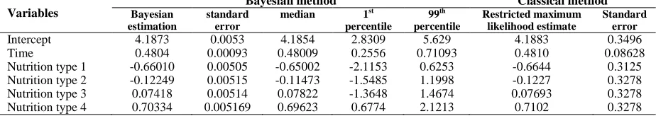
Table 2. Estimation of coefficients using Bayesian and restricted ML methods
Variables
Bayesian method Classical method
Bayesian estimation
standard error
median 1st percentile
99th percentile
Restricted maximum likelihood estimate
The changes resulted from nutrition (random factor) in Bayes estimation and error variance are σ(= 0.98462 and σ)(= 0.111004, respectively. In other words, 89.8% of the total
error is associated with nutrition 44$%
5
%64$% and the
rest is related to other environmental and genetic factors. This ratio is 78.3% in the restricted maximum estimating (Table 1).
According to the estimations above, the coefficients of model (2.1) have been estimated through extracting samples from the bivariate normal distribution the results of which have been indicated in table 2.
Considering table 2, it may be said that in Bayesian method, the credibility range of 98% related to the regression coefficient of time is from 0.2556 to 0.71093. This range indicates that the time factor is effective in normalization of cholesterol; since its coefficient is positive, it illustrates that by passing time, the probability of cholesterol normalization increases and the nutrition type IV has a significant effect on blood cholesterol normalization.
Discussion
The analysis of longitudinal binary responses back to 1969, when Grizel and et al. suggested it (3). Grizel’s model just analyzed complete data. Koch et al. expanded Grizel’s model in order to analyze longitudinal binary responses (4). Woolson and Clarke changed transformed matrix in 1984 and could analyze that data using available software, but the model used by Woolson and Clarke, analyses fixed effect model (5). In 1995, Kazemnejad and Meshkani who expanded this model for fixed and random effects (mixed model) and estimated variance components using Henderson III method, based on the weighted least square (6). Henderson III method is a moment method. Although this is a simple with unbiased estimates, but there is the possibility of zero or negative variance that is futile.
Compare to the classical method, one of the Bayesian difficulties is choosing a prior parameter. We have chosen Jeffries’s prior for variance components which have positive values. Hence, the estimations are positive,
therefore, no choice of negative or zero variance. In the Henderson III method, the same result will not be achieved. Although Bayesian estimation is not unbiased (against the Henderson III method), but there is a discussion about how can an unbiased be a criterion in choosing an estimator. MCMC method has a priority of any sample size with the least standard error.
Conclusion
We see Bayesian method in compare with classical method produce estimations with less standard errors. Using SAS software (SAS Institute Inc.) for estimating parameters is another advantage of this method.
Acknowledgments
Authors acknowledge Shahid Beheshti University of Medical Sciences and Mashhad University of Medical Sciences for Their support.
References
1. Diggle P, Heagerty P, Liang K, Zeger S. Analysis of longitudinal data. Oxford, UK: Oxford University Press; 2013.
2. Little RJA. Statistical analysis with missing data. New York, NY: Wiley; 1987.
3. Cole JWL, Grizzle JE. Applications of multivariate analysis of variance to repeated measurements experiments. Biometrics 1966; 22(4): 810-28.
4. Koch GG, Imrey PB, Reinfurt DW. Linear model analysis of categorical data with incomplete response vectors. Biometrics 1972; 28(3): 663-92.
5. Woolson RF, Clarke WR. Analysis of categorical incomplete longitudinal data. Journal of the Royal Statistical Society 1984; 147(1): 87-99.
6. Kazemnejad A, Meshkani MR. Logit models for random effects in longitudinal binary response with missing values. Journal of Institute of Mathematics & Computer Sciences, 2001; 12(1): 47-53.
bayes methods for data analysis. 2nd ed. New York, NY: Taylor & Francis; 2010.
8. Christensen R. Plane answers to complex questions: the theory of linear models. New York, NY: Springer Science & Business Media, 2000.
9. Hedeker D, Gibbons RD. Longitudinal data analysis. Hoboken, NJ: John Wiley & Sons; 2006.
10.Albert PS. Longitudinal data analysis (repeated measures) in clinical trials. Stat Med 1999; 18(13): 1707-32.
11.Albert I, Jais JP. Gibbs sampler for the logistic model in the analysis of longitudinal binary data. Stat Med 1998; 17(24): 2905-21.
12.Jackman S. Bayesian analysis for the social sciences. Hoboken, NJ: John Wiley & Sons; 2009.
13.Turner RM, Omar RZ, Thompson SG. Bayesian methods of analysis for cluster randomized trials with binary outcome data. Stat Med 2001; 20(3): 453-72.
14.Wolfinger RD, Kass RE. Nonconjugate Bayesian analysis of variance component models. Biometrics 2000; 56(3): 768-74. 15.Kass RE, Wasserman L. The selection of