A New Graph Matching Method for Point-Set
Correspondence using the EM Algorithm and Softassign
Gerard Sanrom`aa,1,∗, Ren´e Alqu´ezarb, Francesc Serratosaa
a
Departament d’Enginyeria Inform`atica i Matem`atiques, Universitat Rovira i Virgili, Av.
Pa¨ısos Catalans, 26 Campus Sescelades, 43007 Tarragona, Spain.
b
Institut de Rob`otica i Inform`atica Industrial, CSIC-UPC, Parc Tecnol`ogic de Barcelona.
C/ Llorens i Artigas 4-6. 08028 Barcelona, Spain.
Abstract
Finding correspondences between two point-sets is a common step in many vision applications (e.g., image matching or shape retrieval). We present a graph matching method to solve the point-set correspondence problem, which is posed as one of mixture modelling. Our mixture model encompasses a model of structural coherence and a model of affine-invariant geometrical er-rors. Instead of absolute positions, the geometrical positions are represented as relative positions of the points with respect to each other. We derive the Expectation-Maximization algorithm for our mixture model. In this way, the graph matching problem is approximated, in a principled way, as a succession of assignment problems which are solved using Softassign. Unlike other ap-proaches, we use a true continuous underlying correspondence variable. We develop effective mechanisms to detect outliers. This is a useful technique for improving results in the presence of clutter. We evaluate the ability of our method to locate proper matches as well as to recognize object categories in a series of registration and recognition experiments. Our method com-pares favourably to other graph matching methods as well as to point-set registration methods and outlier rejectors.
Keywords: correspondence problem, graph matching, affine registration, outlier detection, expectation maximization, softassign
∗Corresponding author
Email addresses: [email protected](Gerard Sanrom`a),[email protected]
(Ren´e Alqu´ezar),[email protected](Francesc Serratosa)
1
1. Introduction
The correspondence problem in computer vision tries to determine which parts of one image correspond to which parts of another image. This prob-lem often arises at the early stages of many computer vision applications such as 3D scene reconstruction, object recognition, pose recovery and image retrieval, among others. So, it is of basic importance to develop effective methods that are both robust -in the sense of being able to deal with noisy measurements- and general -in the sense of having a wide field of application-. The typical steps involved in the solution of the correspondence problem are the following. First, a set of tentative feature matches is computed. These tentative matches can be further refined by a process of outlier rejection that eliminates the spurious correspondences or alternatively, they can be used as starting point of some optimization scheme to find a different, more consistent set.
Tentative correspondences may be computed either on the basis of corre-lation measures or feature-descriptor distances.
Correlation-based strategies compute the matches by means of the simi-larity between the image patches around some interest points. Interest points (that play the role of the images’ parts to be matched) are image locations that can be robustly detected among different instances of the same scene with varying imaging conditions. Interest points can be corners (intersec-tion of two edges) [1] [2] [3], maximum curvature points [4] [5] [6] or isolated points of maximum or minimum local intensity [7].
On the other hand, approaches based on feature-descriptors use the in-formation local at the interest points to compute descriptor-vectors. Those descriptor-vectors are meant to be invariant to geometric and photometric transformations. So that, corresponding areas in different images present low distances between their feature-descriptors. A recent paper by Mikolajczyk and Schmid [8] evaluate some of the most competent approaches.
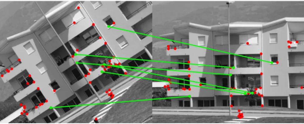
Despite the invariance introduced during the detection/description and the matching phases, the use of local image contents may not suffice to get a reliable result under certain circumstances (e.g., regular textures, multiple instances of a given feature across the images or, large rigid/non-rigid defor-mations). Figure 1 shows an example of a matching by correlation of a scene under rotation and zoom.
Figure 1: Two sample images belonging to the classResid from ref. [9] with superposed Harris corners [1]. The green lines represent the tentative correspondences computed by matching by correlation. The red dots are unmatched points. There are several misplaced correspondences.
It is a standard procedure to exploit the underlying geometry of the prob-lem to enforce the global consistency of the correspondence-set. This is the case of the model fitting paradigm RANSAC [10] which is extensively used in computer vision to reject outliers. It selects random samples of corre-spondences from a tentative set and use them to fit a geometric model to the data. The largest consensus obtained after a number of trials is selected as the inlier class. Another effective outlier rejector is based on a Graph Transformation [11]. This is an iterative process that discards one outlying correspondence at a time, according to a graph-similarity measure. After each iteration, the graphs are reconfigured in order to reflect the new state of the remaining correspondences. The process ends up with two isomorphic graphs and the surviving correspondences constitute the inlier class.
The main drawback of these methods is that their ability to obtain a dense correspondence-set strongly depends on the reliability of the tentative correspondences. Since they are unable either to generate new correspon-dences or to modify the existing ones, an initial correspondence-set with few successes may result in a sparse estimate. This is illustrated in figure 2.
Other approaches such as Iterative Closest Point (ICP) [12] that fall into the optimization field, attempt to simultaneously solve the correspondence and the alignment problem. Despite they are able to modify the correspon-dences at each iteration, simple nearest neighbour association is prone to local minima, specially under bad initial alignment estimates.
Figure 2: The green lines represent the resulting RANSAC inliers from the initial correspondence-set from figure 1. Only a few inliers are found by RANSAC. This may not be suitable in the cases when a more dense correspondence-set is needed.
Attributed Relational Graphs (more generally, graphs) are representa-tional entities allowing for attributes in the nodes and relations among them in the edges. Attributed Graph Matching methods are optimization tech-niques that contemplate these two types of information to compute the matches and therefore, do not rely on simple nearest neighbour association. In the following section, we review the process of solving the correspondence problem in computer vision using graph techniques.
1.1. The Correspondence Problem in Computer Vision using Graphs
The first step at solving the correspondences between two images is to extract their graph representations.
In the case of general images, a commonly adopted representation is to associate feature points to nodes and generate the edge relations following either a Delaunay triangulation [13] or a k-nearest-neighbor strategy [11].
In the case of binary shape images, it is common to extract the graphs us-ing the shapes’ medial axis or skeleton [14] [15]. Some approaches to chinese character recognition represent the strokes in the nodes [16] [17]. However, it is more usual to represent the skeletal end-and-intersection-points in the nodes, and their links in the edges. Some approaches use Shock-graphs [18] [19] [20] or Attributed Skeletal Graphs [21]. These are types of graphs which are closely related to the skeletal representations and therefore, cannot be applied to more general computer vision problems.
Labeling objects of a scene using their relational constraints is at the core of all general-purpose graph-matching algorithms. An early attempt to discrete labeling was by Waltz [22]. Rosenfeld et al. [23] developed a model to relax the Waltz’s discrete labels by means of probabilistic assignments. They introduced the notion of compatibility coefficients and laid the bases of
probabilistic relaxation in graph matching. Hummel and Zucker [24] firmly positioned the probabilistic relaxation into the continuous optimization do-main by demonstrating that finding consistent labellings was equivalent at maximizing a local average consistency functional. Thus, the problem could be solved with standard continuous optimization techniques such as gradi-ent ascgradi-ent. Gold and Rangarajan [25] developed an optimization technique,
Graduated Assignment, specifically designed to the type of objective func-tions used in graph matching. They used a Taylor series expansion to ap-proximate the solution of a quadratic assignment problem by a succession of easier linear assignment problems. They used Softassign [26][27][28] to solve the linear assignment problems in the continuous domain. The key ingredients of their approach were two-way constraints satisfaction and a continuation method to avoid poor local minima.
Another family of approaches, also in the continuous optimization do-main, uses statistical estimation to solve the problem. Christmas et al. [29] derived the complete relaxation algorithm, including the calculation of the compatibility coefficients, following the Maximum A Posteriori (MAP) rule. Hancock et al. [30][31] used cliques, a kind of graph sub-entities, for graph matching. Furthermore, they proposed a new principled way of detecting outliers that consists in measuring the net effects of a node deletion in the retriangulated graph. Accordingly, an outlier is a node that leads to an im-provement in the consistency of the affected cliques after its removal. Nodes are regularly tested for deletion or reinsertion following this criterion.
Hancock et al. [32] [31] formulated the problem of graph matching as one of probability mixture modeling. This can be thought of as a missing data problem where the correspondence indicators are the parameters of the distribution and the corresponding nodes in the model-graph are the hidden variables. They used the Expectation-Maximization (EM) Algorithm [33] to find the Maximum Likelihood (ML) estimate of the correspondence indicators. Hancock et al. [34] [31] presented approaches to jointly solve the correspondence and alignment problems. They did so by exploiting both the geometrical arrangement of the points and their structural relations.
alignment problem, are twofold. On one hand, structural information may contribute to disambiguate the recovery of the alignment (unlike purely geo-metric approaches). On the other hand, geogeo-metrical information may aid to clarify the recovery of the correspondences in the case of structural corruption (unlike structural graph matching approaches).
We present a new graph matching approach aimed at finding the corre-spondences between two sets of coordinate points. The main novelties of our approach are:
• Instead of individual measurements, our approach uses relational infor-mation of two types: structural and geometrical. This contrasts with other approaches that use absolute geometrical positions [31][34].
• It maintains a true continuous underlying correspondence variable through-out all the process. Although there are approaches that relax the discrete assignment constraints through the use of statistical measure-ments, their underlying assignment variable remains discrete [30][31][32][34].
• We face the graph matching problem as one of mixture modelling. To that end, we derive the EM algorithm for our model and approximate the solution as a succession of assignment problems which are solved using Softassign.
• We develop effective mechanisms to detect and remove outliers. This is a useful technique in order to improve the matching results.
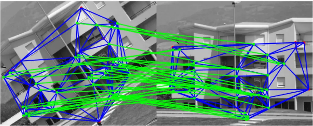
Figure 3 shows the results of applying our method to the previous match-ing example.
Although they are more effective, Graph Matching algorithms are also more computationally demanding than other approaches such as the robust estimator RANSAC. Suboptimal Graph Matching algorithms, such as the ones treated in this paper, often present an O(N4) complexity. However,
Graph Matching algorithms can be very useful at specific moments during a real-time operation, e.g. when the tentative correspondence-sets are insuf-ficient for further refinement or when drastic discontinuities appear in the video flow that cause the tracking algorithms to fail. When these circum-stances are met, it may be advisable to take a couple of seconds in order to conveniently redirect the process. We present computational time results that demonstrate that our algorithm can match a considerable amount of points in an admissible time using a C implementation.
Figure 3: Superposed on the images there are the extracted graphs. Blue lines within each image represent the edges, generated by means of a Delaunay triangulation on the nodes. The nodes correspond to the Harris corners. The green lines represent the resulting correspondences of applying our method, using as starting point the correspondence-set of figure 1. Our approach arrives at a correct dense correspondence-state, while still leaving a few unmatched outliers in both images.
The outline of this paper is as follows. In section 2, we formalize some concepts such as graphs representations and correspondence indicators. The mixture model is presented in section 3. In section 4, we give the details on the optimization procedure using the EM algorithm. The mechanisms for outlier detection are presented in section 5. Before the experimental valida-tion is provided in secvalida-tion 7, we briefly overview some methods related to ours in section 6. Last, discussion about the results and concluding remarks are given in sections 8 and 9.
2. Graphs and Correspondences
Consider two graph representations G = (v, D,p) and H = (w, E,q), extracted from two images (e.g., figure 3).
The node-setsv={va, ∀a∈I} and w={wα, ∀α∈J} contain the symbolic representations of the nodes, where I = 1. . .|v| and J = 1. . .|w| are their index-sets.
The vector-setsp={~pa= (paH, pVa), ∀a∈I}andq={~qα= (qHα, qαV),∀α∈J}, contain the column vectors of the two-dimensional coordinates (horizontal and vertical) of each node.
The adjacency matricesDandEcontain the edge-sets, representing some kind of structural relation between pairs of nodes (e.g., connectivity or spatial
proximity). Hence,Dab =
1 if va and vb are linked by an edge
0 otherwise (the same applies
for Eαβ).
We deal with undirected unweighted graphs. This means that the adja-cency matrices are symmetric (Dab = Dba, ∀a,b∈I) and its elements can only take the {0,1} values. However, our model is also applicable to the directed weighted case.
The variable S represents the state of the correspondences between the node-sets vand w. Therefore, we denote the probability that a nodeva∈v corresponds to a node wα ∈w as saα ∈S.
It is satisfied that
X
α∈J
saα≤1, ∀a∈ I (1)
where the probability of node va being an outlier equals to
1−X
α∈J
saα (2)
2.1. Geometrical Relations
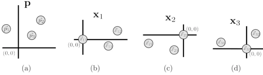
Similarly as it is done with the structural relations, instead of its indi-vidual measurements, our aim is to consider the geometrical relations be-tween pairs of nodes. To that end, we define the new coordinate vectors
~xab = (~pb −~pa), ∀a,b∈I and~yαβ = (~qβ−~qα), ∀α,β∈J, that represent the
coor-dinates of the points~pband~qβ relative to~paand~qα, respectively. Accordingly, we define a new descriptor xa for node va, as the translated positions of the remaining points so that their new origin is at point ~pa, i.e., xa={~xai,i∈I}.
Similarly for graph H,yα ={~yαj,j∈J}. This is illustrated in figure 4. Affine invariance is introduced at the level of node descriptors so, we consider different affine registration parameters Φaα for each possible cor-respondence va → wα. Since geometrical information is used in a rela-tional way, affine registration does not depend on any translation param-eter. Affine registration parameters Φaα are then defined by the 2×2 matrix Φaα = φ11 φ12 φ21 φ22 .
(a) (b) (c) (d)
Figure 4: The entire point-set p(a) and, the descriptors x1(b), x2(c) and x3(d), that
represent the spatial distribution of the point-sets around their new origins~p1,~p2 and~p3,
respectively.
3. A Mixture Model
Our aim is to recover the set of correspondence indicatorsSthat maximize the incomplete likelihood of the relations in the observed graphG. Since the geometrical relations are compared in an affine invariant way, we contemplate the affine registration parameters Φ. Ideally, we seek the correspondence indicators that satisfy
S = arg max ˆ S max ˆ Φ P G|S,ˆ Φˆ (3)
The mixture model reflects the possibility that any single node can be in correspondence with any of the reference nodes. The standard procedure to build likelihood functions for mixture distributions consists in factorizing over the observed data (i.e., observed graph nodes) and summing over the hidden variables (i.e., their corresponding reference nodes). We write,
P (G|S,Φ) =Y
a∈I
X
α∈J
P (va, wα|S,Φaα) (4)
where P (va, wα|S,Φaα) represents the probability that node va corresponds to nodewαgiven the correspondence indicatorsSand the registration param-eters Φaα. We are assuming conditional independence between the observed nodes.
Following a similar development than Luo and Hancock [32] we factor-ize, using the Bayes rules, the conditional likelihood in the right hand side of equation (4) into terms of individual correspondence indicators, in the
following way. P(va, wα|S,Φaα) =Kaα Y b∈I Y β∈J P(va, wα|sbβ,Φaα) (5) where Kaα = 1 P(va|wα,Φaα) |I|×|J |−1 (6) If we assume that the observed nodevais conditionally dependant on the reference node wα and the registration parameters Φaα only in the presence of the correspondence matches S, thenP (va|wα,Φaα) =P (va).
If we assume equiprobable priorsP (va), then we can safely discard these quantities in the maximization of equation (3), since they do not depend neither on S or Φ.
The main aim of equation (5) is to measure the likelihood of the correspon-dence between nodes va ∈vand wα ∈w, by evaluating the compatibility of the pairwise relations emanating from them, by means of the correspondence indicators sbβ.
3.1. A Probability Density Function
In the following, we propose a density function for measuring the condi-tional likelihood of the individual relations in the right hand side of equation (5).
For the sake of clarity, we will define our density function in different stages. First, we will propose separate structural and geometrical models in the case of binary correspondence indicators, i.e., sbβ = {0,1}, ∀b∈I, ∀β∈J. Next, we will fuse these separate relational models into a combined one and, last we will extrapolate to the case of continuous correspondence indicators. Regarding the structural relations, we draw on the model in [32] [34]. It considers that structural errors occur with a constant probabilityPe. This is, given two corresponding pairs of nodes va →wα, vb → wβ, we assume that there will be lack of edge-support (i.e., Dab = 0∨Eαβ = 0) with a constant probability Pe. Accordingly, we define the following likelihood function
P (Dab, Eαβ|sbβ) =
(1−Pe) if sbβ = 1∧Dab= 1∧Eαβ = 1
Pe otherwise (7)
With regards to the geometrical relations we consider that, in the case of correspondence between nodes vb and wβ, an affine-invariant measurement
of the relative point errors P(~xab, ~yαβ|Φaα) (for brevity Paαbβ) is appropriate in gauging the likelihood of the relation ~xab. We use a multivariate Gaussian distribution to model this process. We write
Paαbβ = 1 2π|Σ|1/2 exp −1 2(~xab−Φaα~yαβ) T Σ−1(~xab−Φaα~yαβ) (8)
where Σ is a diagonal variance matrix and, Φaα~yαβ are the transformed co-ordinates ~yαβ according to the affine registration parameters Φaα, a 2×2 matrix of affine scale and rotation parameters. Note that ~xab and ~yαβ are already invariant to translation (figure 4).
In the case of no correspondence between nodes vb and wβ, we assign a constant probability ρ that controls the outlier process (see section 5). Therefore, the conditional likelihood becomes
P (~xab, ~yαβ|sbβ,Φaα) =
Paαbβ if sbβ = 1
ρ if sbβ = 0 (9)
Now it is turn to define a combined measurement for the structural and geometrical likelihoods. To this end, we fuse the densities of equations (7) and (9) into the following expression
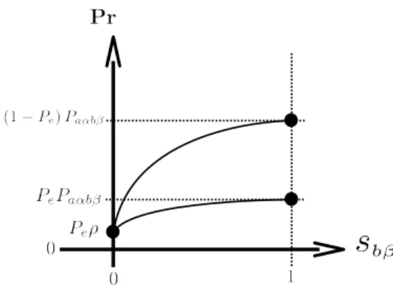
P (va, wα|sbβ,Φaα) = (1−Pe)Paαbβ if sbβ = 1∧(Dab = 1∧Eαβ = 1) PePaαbβ if sbβ = 1∧(Dab = 0∨Eαβ = 0) Peρ if sbβ = 0 (10) The above density function is defined only in the case of binary correspon-dence indicatorssbβ. We extrapolate it to the continuous case by exploiting, as exponential indicators, the conditional expressions of equation (10) in the following way, P(va, wα|sbβ,Φaα) = h (1−Pe)Paαbβ iDabEαβsbβh PePaαbβ i(1−DabEαβ)sbβh Peρ i(1−sbβ) (11)
Figure 5 shows an illustrative plot of the density function of equation (11).
Substituting equation (11) into (5) (and discarding the observed node priors P (va)), the final expression for the likelihood of the correspondence
Figure 5: Density function of equation (11), an extension of the function of equation (10) to continuous correspondence indicators. Each solid curve represent either the case of edge-support (i.e., Dab = 1∧Eαβ = 1) or lack of it (i.e., Dab = 0∨Eαβ = 0). At the
extrema of each curve (i.e., sbβ = {0,1}), represented with black dots (•), we find the
three cases of equation (10).
between nodes va and wα, expressed in the exponential form, is
P (va, wα|S,Φaα) = exp ( X b∈I X β∈J sbβ h DabEαβln 1−Pe Pe + lnPaαbβ ρ i + ln (Peρ) ) (12)
This is, the exponential of a weighted sum of structural and geometrical compatibilities between the pairwise relations emanating from nodes va ∈v and wα ∈ w. The weights sbβ play the role of selecting the proper reference relation (wα, wβ) that it is appropriate in gauging the likelihood of each observed relation (va, vb).
These structural and geometrical coefficients (i.e.,DabEαβln(1−PePe) andln
“Paαbβ
ρ
”
) are equivalent to the compatibility coefficients of the probabilistic relaxation approaches [23][24][29]. In this way, the structural and geometrical compat-ibilities are posed in a principled, balanced footing.
4. Expectation Maximization
The EM algorithm has been previously used by other authors to solve the Graph Matching problem [31] [32]. It is useful to find the parameters that maximize the expected log-likelihood for a mixture distribution. In our case,
we use it to find the correspondence indicators that maximize the expected log-likelihood of the observed relations, given the optimal alignments. From equations (3) and (4), we write,
S = arg max ˆ S ( max ˆ Φaα ( X a∈I ln " X α∈J P va, wα|S,ˆ Φaαˆ #)) (13)
Dempster et al. [33] showed that maximizing the log-likelihood for a mixture distribution is equivalent at maximizing a weighted sum of log-likelihoods, where the weights are the missing data estimates. This is posed as an iterative estimation problem where the new parameters S(n+1) are
up-dated so as to maximize an objective function depending on the previous parameters S(n). Then, the most recent available parametersS(n) are used to
update the missing data estimates that, in turn, weigh the contributions of the log-likelihood functions. Accordingly, this utility measure is denoted
Λ (S(n+1)|S(n)) =X
a∈I
X
α∈J
P(wα|va, S(n),Φaα) lnP (va, wα|S(n+1),Φaα) (14)
where the posterior probabilities of the missing data given the most recent available parameters P (wα|va, S(n),Φaα) weigh the contributions of the con-ditional log-likelihood terms.
The basic idea is to alternate between Expectation and Maximization steps until convergence is reached. The expectation step involves computing the a posterior probabilities of the missing data using the most recent avail-able parameters. In the maximization phase, the parameters are updated in order to maximize the expected log-likelihood of the incomplete data.
4.1. Expectation
In the expectation step, the posterior probabilities of the missing data (i.e., the reference graph measurements wα) are computed using the current parameter estimates S(n).
The posterior probabilities can be expressed in terms of conditional like-lihoods, using the Bayes rule, in the following way
P(wα|va, S(n),Φaα) = P(va, wα|S(n),Φaα) P α′P (va, wα′|S(n),Φaα′) ≡R(n) aα (15)
Substituting our expression of the conditional likelihood of equation (12) into equation (15), the final expression for the posterior probabilities be-comes, R(aαn)= exp ( P b∈I P β∈J s(n) bβDabEαβln 1−Pe Pe +s(n) bβln P aαbβ ρ + ln (Peρ) ) P α′∈J exp ( P b∈I P β∈J s(n) bβDabEα′βln 1−Pe Pe +s(n) bβln P aα′bβ ρ + ln (Peρ) ) (16) 4.2. Maximization
Maximization is done in two steps. First, optimal registration parameters Φaα are computed for each P (va, wα|S,Φaα). Last, global correspondence indicators are updated using the optimal Φaα’s.
4.2.1. Maximum Likelihood Affine Registration Parameters
We are interested in the registration parameters that lead to the maxi-mum likelihood, given the current state of the correspondencesS(n). In other
words, the node descriptors xa and yα must be optimally registered before we can estimate the next correspondence indicators S(n+1). It is important
that the registration do not modify the origins of the node descriptors, since these are the locations of the evaluated nodes va and wα. As consequence, the registration parameters Φaα are a 2× 2 matrix of affine rotation and scaling parameters (without translation).
Therefore, we recover the Maximum Likelihood (ML) registration param-eters Φaα, directly from equation (12). This is,
Φaα = arg max
ˆ Φaα n lnP va, wα|S(n),Φˆaα o = arg max ˆ Φaα ( X b∈I X β∈J s(n) bβln Pˆ aαbβ ρ +DabEαβs(bβn)ln 1−Pe Pe + ln (Peρ) ) (17)
We discard all the terms constant w.r.t the registration parameters and obtain the following equation
Φaα = arg max
ˆ Φaα ( X b∈I X β∈J s(n) bβln ˆ Paαbβ ) (18)
Now, we substitute the geometrical likelihood term by its expression of equation (8). We discard the constant terms of the multivariate Gaussian function and cancel the exponential and the logarithm functions, thus turning the maximization problem into a minimization one, by removing the minus sign of the exponential. We get the following expression
Φaα= arg min
ˆ Φaα ( X b∈I X β∈J s(n) bβ ~xab−Φaαˆ ~yαβ T Σ−1~xab−Φaαˆ ~yαβ ) (19)
We seek the matrix of affine parameters Φaα =
φ11 φ12
φ21 φ22
that minimize the weighted sum of squared Mahalanobis distances between the relative points ~xab and the transformed relative points ˆΦaα~yαβ. The coefficients sbβ weigh the contribution of each pairwise distance in a way that the resulting registration will tend to minimize the distances between the relative positions of those vb and wβ with the larger correspondence indicators.
Further developing equation (19), we obtain the following objective func-tion E =X b∈I X β∈J sbβ h xH ab−φ11yαβH −φ12yαβV 2 /σ2 H+ xV ab−φ21yHαβ−φ22yVαβ 2 /σV2 i (20) where ~xab = (xHab, x V ab) and ~yαβ = yαβH , y V αβ
contain the horizontal and vertical coordinates of vb and wβ relative to va and wα, respectively, and Σ = diag (σ2
H, σ
2
V) is a diagonal matrix of variances.
Minimization of equation (20) w.r.t. the affine parametersφij is done by solving the set of linear equations δE/δφij = 0.
4.2.2. Maximum Likelihood Correspondence Indicators
One of the key points in our work is to approximate the solution of the graph matching problem by means of a succession of easier assignment lems. Following the dynamics of the EM algorithm, each one of these prob-lems is posed using the most recent parameter estimates. As it is done in Graduated Assignment [25], we use the Softassign [26][27][28] to solve the assignment problems in a continuous way. The two main features of the Softassign are that, it allows to adjust the level of discretization of the so-lution by means of a control parameter and, it enforces two-way constraints
by incorporating a method discovered by Sinkhorn [26]. The two-way con-straints guarantee that one node of the observed graph can only be assigned to one node of the reference graph, and vice versa. In the case of continu-ous assignments, this is accomplished by applying alternative row and col-umn normalizations (considering the correspondence variableS as a matrix). Moreover, Softassign allows us to smoothly detect outliers in both sides of the assignment (see section 5).
According to the EM development, we compute the correspondence indi-catorsS(n+1) that maximize the utility measure of equation (14). In our case,
this equals to S(n+1) = arg max ˆ S n ΛSˆ|S(n)o = arg max ˆ S ( X a∈I X α∈J R(n) aα X b∈I X β∈J ˆ sbβ h DabEαβln 1−Pe Pe + lnPaαbβ ρ i + ln (Peρ) ) (21) where R(n)
aα are the missing data estimates.
Rearranging, and dropping the terms constant w.r.t the correspondence indicators, we obtain S(n+1) = arg max ˆ S ( X b∈I X β∈J ˆ sbβ X a∈I X α∈J R(n) aα h DabEαβln 1−Pe Pe + lnPaαbβ ρ i ) (22)
which, as it can be seen in the following expression, presents the same form as an assignment problem [25] S(n+1) = arg max ˆ S ( X b∈I X β∈J ˆ sbβQ(bβn) ) (23) where the Q(n)
bβ are the benefit coefficients for each assignment.
Softassign computes the correspondence indicators in two steps. First, the correspondence indicators are updated with the exponentials of the benefit coefficients
where µis a control parameter. Second, two-way constraints are imposed by alternatively normalizing across rows and columns the matrix of exponenti-ated benefits. This is known as the Sinkhorn normalization and it is applied either until convergence of the normalized matrix or a predefined number of times.
Note that, the correspondence indicators sbβ will tend to discrete values (sbβ ={0,1}) as the control parameter µ of equation (24) approaches to∞. We also apply the Sinkhorn normalization to the posterior probabilities of the missing data so that they are more correlated with the correspondence indicators.
Since the matrices may not be square (i.e., different number of nodes in the observed and reference graphs), in order to fulfill the law of total proba-bility, we complete the Sinkhorn normalization process with a normalization by rows.
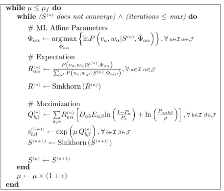
Figure 6 shows the pseudo-code implementation of our method. whileµ≤µf do
while(S(n) does not converge) ∧(iterations ≤max)do
# ML Affine Parameters
Φaα←arg max
ˆ Φaα n lnPva, wα|S(n) ,Φˆaα o ,∀a∈Iα∈J # Expectation R(n) aα← P(va,wα|S(n),Φaα) P α′P(va,wα′|S(n),Φaα′) ,∀a∈Iα∈J R(n)←Sinkhorn (R(n)) # Maximization Q(n) bβ ← P a,α R(n) aα h DabEαβln1−Pe Pe + lnPaαbβ ρ i ,∀b∈Iβ∈J s(n+1) bβ ←exp µ Q(n) bβ ,∀b∈Iβ∈J S(n+1)←Sinkhorn (S(n+1)) S(n)←S(n+1) end µ←µ×(1 +ǫ) end
Figure 6: The outer loop gradually increase the Softassign parameterµ, thereby pushing from continuous to discrete solutions. This reduces the chances of getting trapped in local minima [25]. The body contains the pseudo-code of the E and M steps. Each iteration of the inner loop performs one step of the EM algorithm.
5. Outlier Detection
A node in one graph is considered to be an outlier if it has no correspon-dent node in the other graph.
Consider, for example, the case of figure 3. The rightmost nodes in the right image are outliers originated from the detection of features in the non-overlapping parts of the images. On the other hand, the unmatched nodes in the overlapping parts are outliers originated by differences in the feature detection patterns.
Outliers can dramatically affect the performance of a matching and there-fore, it is important to develop techniques aimed at minimizing their influence [35].
According to our purposes, a node vb ∈v (orwβ ∈w) will be considered an outlier to the extent that there is no node wβ, ∀β∈J (or vb,∀b∈I) which
presents a matching benefit Q(n)
bβ above a given threshold.
From equations (22) and (23), the benefit values have the following ex-pression Q(n) bβ = X a∈I X α∈J R(n) aα h DabEαβln 1−Pe Pe + lnPaαbβ ρ i (25)
Note that, the value of ρ controls whether the geometrical compatibility term contributes either positively (i.e., ρ < Paαbβ) or negatively (i.e., ρ >
Paαbβ) to the benefit measure.
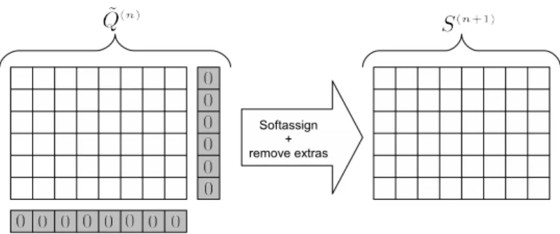
We model the outlier detection process as an assignment to (or from) the null node. We consider that the null node has no edges at all and, all the geometrical terms Paαbβ involving it are equal to ρ. Under these considerations, the benefit values of equation (25) corresponding to the null assignments are equal to zero. We therefore create an augmented benefit matrix ˜Q(n) by adding toQ(n) an extra row and column of zeros. This extra
row and column represent the benefits of thenull assignments (i.e.,Qb∅,∀b∈I
and Q∅β, ∀β∈J).
We apply the Softassign (exponentiation and Sinkhorn normalization) to the augmented benefit matrix ˜Q(n). When performing Sinkhorn
normalitza-tion we keep in mind that the null assignments are special cases that only satisfy one-way constraints. This is, there may be multiple assignments to
null in both graphs. Finally, the extra row and column are removed leading to the resulting matrix of correspondence parameters S(n+1). This process is
Figure 7: The Softassign and outlier detection process.
As the control parameter µ of the Softassing increases, the rows and columns of S(n+1) associated to the outlier nodes, tend to zero. This fact
reduces the influence of these nodes in the maximization phases of the next iteration that, in turn, lead to even lower benefits, and so on.
It is now turn to define the value of the constant ρ. Since ρ is to be compared with Paαbβ, it is convenient to define it in terms of a multivariate Gaussian measurement of a distance threshold. This is,
ρ= 1 2π|Σ|1/2 exp −1 2d~ TΣ−1d~ (26) where Σ = diag (σH2, σ 2
V) is the same diagonal variance matrix as we use in
equation (8) and d~ = (dH, dV) is a column vector with the horizontal and
vertical thresholding distances.
Cancelling the constant terms in the numerator and denominator of the geometrical compatibility term and expressing the thresholding distances as a quantity proportional to the standard deviations of the data, (i.e., d~ = (NσH, NσV)), the expression ofρ to be compared with Paαbβ is
ρ= exp ( −1 2 " NσH σH 2 + NσV σV 2#) = exp −N2 (27)
So, we define ρ as a function of the number N of standard deviations permitted in the registration errors, in order to consider a plausible corre-spondence.
6. Related Methods
In this section we briefly overview to existing methods related to ours that are used in the experiments.
Cross and Hancock perform graph matching with aDual-Step EM algo-rithm [31]. They update alignment parameters according to the following rule. Φ(n+1) = arg max ˆ Φ X a∈I X α∈J P(wα|va,Φ(n))ζaα(f(n)) lnP va, wα|Φˆ (28)
where ζaα(f(n)) is the expected value for the assignment probabilities re-garding the structural consistence of the mappings defined by the correspon-dences f(n), Pv
a, wα|Φˆ
is a multivariate Gaussian measurement of the point position errors given the alignment parameters and, P (wα|va,Φ(n)) is the posterior probability term computed in the E-step.
Correspondence variables are estimated in a discrete way with the follow-ing Maximum a Posteriori rule.
f(n+1)
(a) = arg max α
P (wα|va,Φ(n))ζaα(f(n)) (29)
Luo and Hancock’s present aUnified framework for alignment and corre-spondence [34] that maximizes a cross-entropy measure in an EM-like fashion. They estimate Maximum Likelihood alignment and correspondence parame-ters according to the following rules.
Φ(n+1) = arg max ˆ Φ X a∈I X α∈J Q(n) aαlnP va, wα|Φˆ (30) and S(n+1) = arg max ˆ S X a∈I X α∈J P(n) aαlnQ va, wα|Sˆ (31) where Q(n)
aα and Paα(n) are the posterior probability terms according to struc-tural and positional observations and P (•) andQ(•) are the corresponding probability density functions. Correspondence variables are updated in a discrete way.
7. Experiments and Results
We assess the performance of our method in terms of registration accuracy and recognition ability.
We have roughly set the value ofρ= exp (−1.62) for our method in all the
experiments. We have not found this parameter to be specially application dependant since this same value has offered a fair performance in all the variety of experiments presented.
The parameters for the rest of the methods have been likewise set so as to show a good performance. We have tried to be as efficient as possible in the implementations of all the methods. Unless otherwise noted, all the computational time results refer to MatlabR run-times. All the experiments
have been conducted on an IntelR XeonR CPU E5310 at 1.60GHz. 7.1. Registration Experiments
These experiments are aimed at testing both the ability of our model to discriminate correct matching hypothesis as well as the accuracy of the optimization method to locate them.
Performance is assessed by either the correct correspondence rate or the
mean projection error depending on whether the graphs are synthetically generated (with known ground truth correspondences) or extracted from real images (with known ground truth homography). We compare to other graph matching methods as well as to known point-set registration methods and outlier rejectors.
The parameter Pe is more application dependant than ρ since it estab-lishes the scale of the structural contribution of our model which is to be added to the geometric contribution in order to set up the consistency mea-sure of equation (25). Specifically, the value of the structural contribution depends on this scale parameter as well as the mean node degree (i.e., the mean number of incident edges upon each node).
All the graphs used in this section have been generated by means of Delaunay triangulations over point-sets, where each point has been assigned to a node. We have conducted matching experiments on randomly generated graphs and have experimentally found that a value ofPe= 0.03 performs well for this type of graphs. Therefore, we have used this value for our method in all the experiments in this section.
This section is divided as follows. In sections 7.1.1 and 7.1.2 we use synthetic graphs to evaluate specific aspects of our model. In section 7.1.3
we use real images.
7.1.1. Synthetic Non-Rigid Deformations
In the next set of experiments we evaluate the matching ability in the presence of non-rigid deformations. We have matched randomly generated patterns of 15 points with deformed versions of themselves. Deformations have been introduced by applying random Gaussian noise to the coordinate positions of the points.
In the synthetic experiments we assess the performance of each method through the correct correspondence rate. To see how this performance mea-sure is related to our model we meamea-sure the ratio LEM−Sof t/Lgtr, between the value of the log-likelihood function at the solution found by the EM algorithm and that at the ground truth matching.
From equation (4) the expression of log-likelihood function according to our model is the following.
L=X a∈I ln " X α∈J P va, wα|S,ˆ Φaαˆ # (32)
Figure 8 shows that even though there is an increasing trend in the dis-agreement between the model hypothesis and the established ground truth as the deformation increases, such a disagreement remains close to the optimum value of 1 for deformations up to 20%.
We have compared the correct correspondence rates of our method ( EM-Soft) to that of the graph matching + point-set alignment methodsDual-Step
and Unified. The Dual-Step has been implemented with an affine geomet-rical model as well as the capability of detecting outliers. Such an outliers-detection capability increases considerably its required computational time but, evaluating the performance of this feature is an important aspect in our experiments. All the approaches have been initialized with the resulting correspondences of a simple nearest neighbour association. Figure 9 shows the correct correspondence rates with respect to the amount of noise. The mean computational times are: 14.6 sec. (EM-Soft), 124.5 sec. (Dual-Step) and 0.91 sec. (Unified).
The computational time obtained with a C implementation of our method is 0.24 sec.
0.02 0.04 0.06 0.08 0.1 0.12 0.14 0.16 0.18 0.2 0.995 1 1.005 1.01 1.015 1.02 1.025
Amount of noise proportional to the standard deviation of the data
Disagreement ratio
Figure 8: Ratio of the log-likelihood of the suboptimal solution found by our method to that of the ground truth solution, according to our model. As the deformation increases the likelihood of the ground truth solution falls below other (partially incorrect) solutions. Each location on the plots is the mean of 25 experiments (5 random patterns of points by 5 random deformations). 0.020 0.04 0.06 0.08 0.1 0.12 0.14 0.16 0.18 0.2 0.1 0.2 0.3 0.4 0.5 0.6 0.7 0.8 0.9 1
Proportion of noise w.r.t standard deviation of the data
Correct correspondence rate
EM−Soft Dual−Step Unified
Figure 9: Correct correspondence rate with respect to the amount of noise in the point positions (expressed proportionally to the variance of the data). Each location on the plots is the mean of 25 experiments (5 random patterns of points by 5 random deformations).
7.1.2. Synthetic Addition of Random Points
The next set of experiments evaluates the matching ability in the presence of outliers. We have randomly added outlying points (with no correspondence in the other side) tobothsynthetic patterns of 15 points. We have preserved a proportion of ground-level non-rigid noise of 0.02 between the inliers of both patterns. In order to contribute positively to the correct correspondence rate,
outliers must not be matched to any point while, inliers must be assigned to its corresponding counterpart. The approaches compared in this experiment are those with explicit outlier detection mechanisms. These are RANSAC
(affine) [10], Graph Transformation Matching (GTM) [11] and Dual-Step
[31].
GTM is a powerful outlier rejector based on a graph transformation that holds a very intuitive idea. We use the same strategy as in [11] consisting in using k-NN graphs with k = 5 instead of Delaunay triangulations in order to present the results for the GTM method. However, similar results are obtained using Delaunay triangulations.
All the methods have been initialized with the resulting correspondences of a simple nearest neighbour association. Figure 10 shows the correct cor-respondence rate with respect to the number of outliers and figure 11 shows the computational times.
1 2 3 4 5 6 7 8 9 10 0 0.1 0.2 0.3 0.4 0.5 0.6 0.7 0.8 0.9 1
Number of outliers added in both point−sets
Correct correspondence rate
EM−Soft Dual−Step RANSAC GTM
Figure 10: Correct correspondence rate with respect to the number of outliers in each side. Each location is the mean of 125 experiments (5 random inlier patterns by 5 random outlier patterns by 5 random ground-level non-rigid noise).
7.1.3. Real Images
We have performed registration experiments on real images from the database in ref. [9]. Point-sets have been extracted with the Harris op-erator [1]. Each pair of images shows two scenes related by either a zoom or a zoom + rotation. They belong to the classes Resid, Boat, New York and
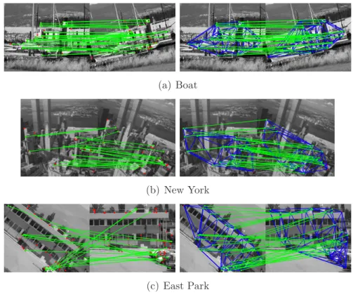
East Park. All the approaches use the same parameters as in the previous section. Figures 3 and 12 show the resulting correspondences found by our method as well as the tentative correspondences used as starting point.
1 2 3 4 5 6 7 8 9 10 10−3 10−2 10−1 100 101 102 103 Number of outliers
Computational time in seconds (logarithmic scale)
EM−Soft Dual−Step RANSAC GTM
Figure 11: Plots of the computational times with respect to the number of outliers. The time (vertical) axis is in logarithmic scale.
(a) Boat
(b) New York
(c) East Park
Figure 12: Right column shows the results of our method using the matching by correlation results (left column) as starting point.
We have compared all the methods with outlier detection capabilities of the previous section. The graph-based approaches have been initialized with the matching by correlation results (Corr). We have used the matching by correlation implementation found in ref. [36]. In order to avoid the sparsity problem mentioned in figure 2, we have applied ICP [12] to the correlation results, as a previous step to the outlier rejectors RANSAC and GTM.
From the resulting correspondences, we have estimated the corresponding homographies with the DLT algorithm [37]. Since the ground truth homog-raphy between each pair of images is available, we have measured the mean projection error (MPE) of the feature-points in the origin images. Table 1 shows the mean projection errors as well as the proportion of matched points in the origin images. Table 2 shows the computational times in seconds. Ta-ble 4 shows the computational times of the Matlab and C implementations of our method.
In order to show how methods benefit from outlier rejection in a real world application, we have repeated the above experiments using the Unified
method and the pure structural method Graduated Assignment ( GradAs-sig) [25], both without explicit outlier rejection capabilities. We have also added modified versions of EM-Soft and Dual-Step so that outlier rejection is disabled (marked with an asterisk). Table 3 shows the results.
7.2. Recognition Experiments
In this section we assess the recognition ability of the underlying model used in our graph matching method in a series of shape retrieval experiments on the GREC database [38] and a database of 25 shapes. In these experi-ments, the structure of the graphs has been given rise by the morphology of the objects.
Due to numerical reasons, lower values ofPe are needed in the case of this morphologically-induced graphs than in the case of Delaunay triangulations. This is because in this case, resulting graphs are sparser and therefore struc-tural contributions under equation (25) need to be amplified so as to play a role comparable to the geometric contributions. We have used the first 5 graphs from each class of the GREC database in order to tune the param-eters of all the methods. Due to the similar nature of the graphs in both databases and to the lack of examples in the 25-shapes database in order to perform training, we have used the same parameters in both databases. We have used a value of Pe = 3·10−4 for our method.
Resid Boat New York East Park
Method MPE % MPE % MPE % MPE %
Corr 835 27 24.5 76 31 67 463 43 ICP 40.3 87 21 100 19.4 100 88 100 EM-Soft 1.5 69 0.68 72 0.69 91 1.13 75 Dual-Step 1.3 72 1.7 62 0.7 91 153 25 ICP+RANSAC 12.3 54 10.7 64 10.9 76 98 41 ICP+GTM 32.5 61 10.5 70 2.9 70 327 45
Table 1: Mean Projection Error (MPE) and percentage of matched points in the origin images (%).
Method Resid Boat New York East Park
Corr 0.54 0.55 0.26 0.55 ICP 0.22 0.18 0.13 0.2 EM-Soft 378 449 73 438 Dual-Step 3616 3794 1429 3027 ICP+RANSAC 0.29 0.24 0.18 0.3 ICP+GTM 0.23 0.25 0.17 0.27
Table 2: Computational times (in seconds). The number of points of the origin (N1) and destination (N2) images in each case are: Resid N1 = 55, N2 = 48;Boat N1 = 50, N2 =
61;New York N1 = 34, N2 = 34;East Park N1 = 44, N2 = 67.
Resid Boat New York East Park
Method MPE % MPE % MPE % MPE %
EM-Soft∗ 2619 87 25.3 100 23.9 100 56.8 95
Dual-Step∗ 26.2 83 19.5 100 1.15 91 332 100
Unified 39.8 69 12.3 86 3.04 88 1104 75
GradAssig 174 85 60.8 100 14.8 94 1716 100
Table 3: Mean Projection Error (MPE) and percentage of matched points (%) obtained without outlier rejection mechanisms.
Method Resid Boat New York East Park
EM-Soft (Matlab) 378 449 73 438
EM-Soft (C) 15.5 19.5 2.1 19.1
Given a query graphG, we compute its similarity to a database graphH
using the following measure
FGH = maxSˆ F G, H; ˆS max (FGG,FHH) (33)
where, FG, H; ˆS= lnP G|S,ˆ Φ is the incomplete log-likelihood of the observed graphG, assumingHas the missing data graph;FGG=F(G, G;IG) and FHH = F(H, H;IH), being IG and IH the identity correspondence indicators defining self-matchings. This results in a normalized measure
FGH ∈ [0,1] that equals to one in the case of a self-matching between two identical graphs and, moves towards zero as they become different.
Note that the maximization in the numerator of equation (33) has the same form as the log-likelihood maximization of equation (13) performed by our EM algorithm (section 4).
Performance is assessed through precision-recall plots. We compute the pairwise similarities between all the graphs in the database thus obtaining, for each query graph, a list of retrievals ordered by similarity. Suppose that our database containsCclasses withN graphs each. We can define a retrieval of depth ras the firstr graphs from each ordered list. Note that the number of elements retrieved by a such an operation is rCN.
Precision is then defined as the fraction of retrieved graphs that are rel-evant in a retrieval of depth r. This is,
precision = #relevant (r)
rCN (34)
where #relevant (r) is the number of retrieved graphs that agree with the class of their respective queries, in a retrieval of depth r.
Recall is defined as the fraction of the relevant graphs that are successfully retrieved by retrieval of depth r. This is,
recall = #relevant (r)
CN2 (35)
where CN2 is the maximum number of relevant graphs possible.
7.2.1. GREC Graphs
We have performed retrieval experiments on the GREC subset of the IAM Graph Database Repository [38]. This subset is composed by 22 classes of 25 graphs each. Figure 13 shows an example graph of each class. Some
Figure 13: An example graph of each class of the GREC database [38]. Nodes are repre-sented as red dots, while edges as blue lines.
classes show considerable inter-class similarities as well as significant intra-class variations such as missing or extra nodes, non-rigid deformations, scale differences and structural disruptions. See for example, the graphs in figure 14.
(a) Class 7 (b) Class 7 (c) Class 6
Figure 14: Compared in an affine-invariant way, graphs 14(a) and 14(c) show a similar node-set arrangement, although they are from different classes. They present however, slight differences between their structure. On the other hand, although graphs 14(a) and 14(b) are from the same class, we can see missing and extra nodes with respect to each other, while still having some differences between their structure. With these considerations, classification is not straightforward.
We have compared our method (EM-Soft) to the purely structural method
GradAssig and the geometric + structural methods Dual-Step [31] and Uni-fied [34]. We have included two additional pure geometric methods in order to provide evidence of the benefits of the combined methods. On one hand, we have used our method with an ambiguous structural model (i.e.,Pe= 0.5). On the other hand, we have implemented a point-set registration algorithm (EM-reg) using the following EM update rule.
Φ(n+1) = arg max ˆ P hi X a∈I X α∈J P (wα|va,Φ(n)) lnP va, wα|Φˆ (36) whereP va, wα|Φˆ
is a multivariate Gaussian function of the point-position errors given the alignment parameters.
For each method, we have used the equivalent analog of the normal-ized similarity measure of equation (33) according to their models. All the approaches have been initialized by the tentative correspondences found as explained in appendix A. The methods that do not use correspondence pa-rameters have been initialized by the alignment papa-rameters that minimize the pairwise point-position errors according to the aforementioned correspon-dences.
Figure 15 shows the precision-recall plots obtained by varying the depth of the retrieval from 1 to 550 (the total number of graphs in the database).
0 0.1 0.2 0.3 0.4 0.5 0.6 0.7 0.8 0.9 1 0 0.1 0.2 0.3 0.4 0.5 0.6 0.7 0.8 0.9 1 Recall Precision EM−Soft EM−Soft (P e=0.5) Dual−Step Unified EM−reg GradAssig
7.2.2. 25 Shapes Database
We have performed retrieval experiments on the database of 25 binary shape images of figure 16. Our aim here is to evaluate the recognition
abil-Figure 16: This database is divided into 6 classes: Shark(5 instances),Plane(4 instances),
Gen (3 instances), Hand (5 instances),Rabbit (4 instances) andTool (4 instances).
ities of several general-purpose graph matching approaches. Therefore, we have not used databases containing more specific types of deformations such as articulations because of the limitations imposed by the affine model as-sumptions.
We have used the skeleton pruning approach by Bai and Latecki [39] in order to obtain the skeletal representations. Graphs have been generated by placing the nodes at the end and intersection skeletal points and, the edges so as to fit to the rest of body of the skeleton. Figure 17 shows the graphs extracted from the above database.
All the approaches have been initialized with the tentative correspon-dences found as explained in appendix A.
We have implemented an affine-invariant template matching method in order to evaluate the benefits of using the structural abstractions instead of using directly the binary images. We evaluate the similarity between two registered binary images on the basis of their overlapping shape areas. Affine registration of the binary images is performed according to the tentative correspondences found by the method in appendix A.
Figure 18 shows the precision-recall plots of the graph matching ap-proaches EM-Soft, Dual-Step and Unified and, the affine-invariant template matching (TM).
Figure 17: Graphs generated from the skeletons of the 25 shapes of figure 16. 0.2 0.3 0.4 0.5 0.6 0.7 0.8 0.9 1 0.1 0.2 0.3 0.4 0.5 0.6 0.7 0.8 0.9 1 EM−Soft Dual−Step Unified TM
Figure 18: Precision-recall plots in the 25-shapes database.
8. Discussion
In the matching experiments under non-rigid deformations our method has shown to be the most effective among the compared graph-matching methods. Moreover, it shows a computational time in the typical range of the graph-matching methods. Dual-Step obtains a higher correct correspondence rate than Unified. However, its computational time is higher as well.
The matching experiments in the presence of outliers show that our method outperforms the compared ones. Dual-Step performs as effectively as RANSAC. Moreover, while outlier rejectors are specifically designed for these type of experiments, Dual-Step has a wider applicability.
The matching experiments on real images show that our method performs generally better than the others. Dual-Step performs, in most cases, similarly as ours but with higher computational times. It is worth mentioning that the considerable computational times required by Dual-Step are mainly due to the bottleneck that represents its outlier detection scheme. The graph-matching methods generally find more dense correspondence-sets. The en-semblesICP+RANSAC and ICP+GTM do not perform as effectively as the graph-matching methods but they do it faster.
Furthermore, we show how different methods benefit from outlier rejection in a real world application.
The efficiency shown by the C implementation of our method suggests that, while the outlier rejectors are appropriate for a regular real-time op-eration, it is feasible to use our method in specific moments when more effectiveness is required.
The dictionary-based structural model of theDual-Step [31] has demon-strated to be the most effective in the retrieval experiments on the GREC database. Our method shows a performance decrease with respect to Dual-Step. Unified is unable to deal with the type of graphs used in this experi-ment.
Neither the pure geometric methods nor the pure structural ( GradAs-sig) are as accurate asDual-Step and EM-Soft in the precision-recall scores. This demonstrates the benefits of combining both sources of information as opposed to using them separately. Particularly revealing of this fact is the comparison between the two versions of our method.
In the 25-shapes database the proposed method and theDual-Stepobtain similar scores. The affine-invariant template matching method only retrieves correctly the most similar instances of each class. As we increment the depth of the retrieval and more significant intra-class variations appear, the direct comparison of templates experiments a decrease in performance with respect to our structural approach. This shows the benefits of using structural repre-sentations as opposed to template-based strategies in the present application. The limitations of the affine model assumptions prevents us from using shape databases presenting further deformations such as larger articulations.
9. Conclusions
We have presented a graph matching method aimed at solving the point-set correspondence problem. Our model accounts for relative structural and
geometrical measurements which keep parallelism with the compatibility co-efficients of the Probabilistic Relaxation approaches. This contrasts with other approaches that use absolute coordinate positions [31][34]. Unlike other approaches [31][34][32][30], our underlying correspondence variable is contin-uous. To that end, we use Softassign to solve the individual assignment problems thus, enforcing two-way constraints as well as being able to con-trol the level of discretization of the solution. Moreover, gradually pushing from continuous to discrete states reduces the chances of getting trapped in local minima [25]. We develop mechanisms to smoothly detect and remove outliers.
In contrast to other approaches such as Unified and Dual-Step, the pro-posed approach has the distinguished properties that it uses Softassign to estimate the continuous correspondence indicators as well as it is based on a model of relational geometrical measurements. Such properties demon-strate to confer the proposed approach a better performance in most of the experiments presented.
Our method is controlled by two parameters, namely, an outlying thresh-old probability ρand a probability of structural errorPe. We have not found any particular dependence of the parameter ρ to a specific application and hence, we have used the same value in all the experiments. On the contrary, the parameter Pe scales the contribution of the structural component of our model which is to be compared to the geometric part. Since the value of the structural contribution depends on both this scaling factor and the mean de-gree of the nodes in the graphs, we have found a dependence of this parameter to the type of graphs used. Therefore, we have used two different values for graphs generated from Delaunay triangulations and morphologically-induced graphs. As far as we know, this dependence does not go further than to the types of graph-representations used.
Appendix A
The following is an adaptation of the Belongie et al.’s shape contexts [40] in order to match point-sets regardless of their orientations. Given two point-sets (in our case, the positions of the nodes), p = {~pa},∀a∈I and q={~qα}, ∀α∈J, we arbitrarily choose one of them (e.g.,q) and createM
distributed along the range [0. . .360] degrees2. We therefore obtain the
sub-sets qm,m∈[1...M], corresponding to M different orientations of q. Next, we
compute the shape contexts, a kind of descriptor (log-polar histograms) that, for each point, encodes how the rest of the points are distributed around it. We do it for theM+ 1 point-setspandqm,m∈[1...M]. Using theχ2 test
statis-tic between the shape contexts [40], we compute theM matrices of matching costs Cm. Thus, Cm
aα indicates the cost of matching the point ~pa∈ p to the point ~qm
α ∈ qm. By applying the Hungarian algorithm [41] to each Cm, we compute the optimal assignments fm:I → J from the points in p to those in each one of the qm’s. We choose as the prevailing orientation m, the one with the minimum matching cost, i.e., m= arg minmˆ
n P Cmˆ a,fmˆ(a) o and, the resulting correspondences are those defined by fm.
Acknowledgements
This research is supported by Consolider Ingenio 2010 (CSD2007-00018), by the CICYT (DPI 2010-17112) and by project DPI-2010-18449.
References
[1] C. Harris, M. Stephens, A combined corner and edge detection, in: Pro-ceedings of The Fourth Alvey Vision Conference, 1988, pp. 147–151. [2] J. Shi, C. Tomasi, Good features to track, in: IEEE Conference on
Computer Vision and Pattern Recognition (CVPR’94), Seattle, 1994. [3] C. Tomasi, T. Kanade, Detection and tracking of point features, Tech.
Rep. CMU-CS-91-132, Carnegie Mellon University (April 1991).
[4] L. Kitchen, A. Rosenfeld, Gray-level corner detection, Pattern Recogni-tion Letters 1 (2) (1982) 95–102.
[5] L. Koenderink, W. Richards, Two-dimensional curvature operators, Journal of the Optical Society of America: Series A 5 (7) (1988) 1136– 1141.
2
[6] W. Han, M. Brady, Real-time corner detection algorithm for motion estimation, Image and Vision Computing (1995) 695–703.
[7] E. Rosten, T. Drummond, Machine learning for high-speed corner de-tection, in: In European Conference on Computer Vision, Vol. 1, 2006, pp. 430–443.
[8] K. Mikolajczyk, C. Schmid, A performance evaluation of local descrip-tors, IEEE Transactions on Pattern Analysis and Machine Intelligence 27 (10) (2005) 1615–1630.
[9] http://www.featurespace.org/.
[10] M. A. Fischler, R. C. Bolles, Random sample consensus: a paradigm for model fitting with applications to image analysis and automated cartography, Comunications of the ACM 24 (6) (1981) 381–395.
[11] W. Aguilar, Y. Frauel, F. Escolano, M. E. Martinez-Perez, A robust graph transformation matching for non-rigid registration, Image and Vision Computing 27 (2009) 897–910.
[12] Z. Zhang, Iterative point matching for registration of free-form curves and surfaces, International Journal of Computer Vision 13 (2) (1994) 119–152.
[13] R. Wilson, A. Cross, E. Hancock, Structural matching with active tri-angulations, Computer Vision and Image Understanding 72 (1) (1998) 21–38.
[14] H. Blum, A transformation for extracting new descriptors of shape, in: Models for the Perception of Speech and Visual Form, MIT Press, 1967, pp. 363–380.
[15] W.-B. Goh, Strategies for shape matching using skeletons, Computer Vision and Image Understanding 110 (3) (2008) 326–345.
[16] K. Chan, Y. Cheung, Fuzzy-attribute graph with application to chinese character-recognition, IEEE Transactions on Systems Man and Cyber-netics 22 (2) (1992) 402–410.
[17] P. Suganthan, H. Yan, Recognition of handprinted chinese characters by constrained graph matching, Image and Vision Computing 16 (3) (1998) 191–201.
[18] K. Siddiqi, A. Shokoufandeh, S. J. Dickinson, S. W. Zucker, Shock graphs and shape matching, International Journal of Computer Vision. [19] T. Sebastian, P. Klein, B. Kimia, Recognition of shapes by editing their shock graphs, IEEE Transactions on Pattern Analysis and Machine In-telligence 26 (5) (2004) 550–571.
[20] A. Torsello, E. Hancock, A skeletal measure of 2d shape similarity, Com-puter Vision and Image Understanding 95 (1) (2004) 1–29.
[21] C. Di Ruberto, Recognition of shapes by attributed skeletal graphs, Pattern Recognition 37 (1) (2004) 21–31.
[22] D. Waltz, Understanding line drawings of scenes with shadows, in: The Psychology of Computer Vision, McGraw-Hill, 1975, p. pages.
[23] A. Rosenfeld, R. A. Hummel, S. W. Zucker, Scene labelling by relaxation operations, IEEE Transactions on Systems, Man and Cybernetics (6) (1976) 420–433.
[24] R. A. Hummel, S. W. Zucker, On the foundations of relaxation labling processes, IEEE Transactions on Pattern Analysis and Machine Intelli-gence 5 (3) (1983) 267–287.
[25] S. Gold, A. Rangarajan, A graduated assignment algorithm for graph matching, IEEE Transactions on Pattern Analysis and Machine Intelli-gence 18 (4).
[26] R. Sinkhorn, Relationship between arbitrary positive matrices + doubly stochastic matrices, Annals of Mathematical Statistics 35 (2) (1964) 876–&.
[27] H. Chui, A. Rangarajan, A new point matching algorithm for non-rigid registration, Computer Vision and Image Understanding 89 (2-3) (2003) 114–141.
[28] A. Rangarajan, S. Gold, E. Mjolsness, A novel optimizing network archi-tecture with applications, Neural Computation 8 (5) (1996) 1041–1060.
[29] W. Christmas, J. Kittler, M. Petrou, Structural matching in computer vision using probabilistic relaxation, IEEE Transactions on Pattern Analysis and Machine Intelligence 17 (8) (1995) 749–764.
[30] R. Wilson, E. Hancock, Structural matching by discrete relaxation, IEEE Transactions on Pattern Analysis and Machine Intelligence 19 (6) (1997) 634–648.
[31] A. Cross, E. Hancock, Graph matching with a dual-step em algorithm, IEEE Transactions on Pattern Analysis and Machine Intelligence 20 (11) (1998) 1236–1253.
[32] B. Luo, E. R. Hancock, Structural graph matching using the em algo-rithm and singular value decomposition, IEEE Transactions on Pattern Analysis and Machine Intelligence 23 (10).
[33] A. P. Dempster, N. M. Laird, D. B. Rubin, Maximum likelihood from incomplete data via the em algorithm, Journal of the Royal Statistical Society, Series B 39 (1) (1977) 1–38.
[34] B. Luo, E. Hancock, A unified framework for alignment and correspon-dence, Computer Vision and Image Understanding 92 (1) (2003) 26–55. [35] M. Black, A. Rangarajan, On the unification of line processes, outlier rejection, and robust statistics with applications in early vision, Inter-national Journal of Computer Vision 19 (1) (1996) 57–91.
[36] http://www.csse.uwa.edu.au/~pk/Research/MatlabFns/.
[37] R. Hartley, A. Zisserman, Multiple View Geometry in Computer Vision, Cambridge University Press, 2003.
[38] K. Riesen, H. Bunke, Iam graph database repository for graph based pattern recognition and machine learning, in: Structural, Syntactic, and Statistical Pattern Recognition, Vol. 5342 of Lecture Notes in Computer Science, 2008, pp. 287–297.
[39] X. Bai, L. J. Latecki, W.-Y. Liu, Skeleton pruning by contour parti-tioning with discrete curve evolution, IEEE Transactions on Pattern Analysis and Machine Intelligence 29 (3) (2007) 449–462.
[40] S. Belongie, J. Malik, J. Puzicha, Shape matching and object recogni-tion using shape contexts, IEEE Trans. Pattern Analysis and Machine Intelligence. 24 (4) (2002) 509–522.
[41] J. Munkres, Algorithms for the assignment and transportation problems, Journal of the Society for Industrial and Applied Mathematics 5 (1) (1957) 32–38.
Gerard Sanrom`a obtained his computer science engi-neering degree at Universitat Rovira i Virgili (Tarragona Spain) in 2004. He is now a Ph.D. student. His main areas of interest are computer vision, structural pattern recognition, graph matching and shape analysis.
Rene Alqu´ezar received the licentiate and Ph.D. degrees in Computer Science from the Universitat Polit`ecnica de Catalunya (UPC), Barcelona, in 1986 and 1997, respectively. From 1987 to 1991 he was with the Spanish company NTE as technical manager of R&D projects on image processing applications for the European Space Agency (ESA). From 1991 to 1994 he was with the Institut de Cibernetica, Barcelona, holding a pre-doctoral research grant from the Government of Catalonia. He joined the Department of Llenguatges i Sistemes Informatics, UPC, in 1994 as an assis-tant professor, and since March 2001 he has been an associate professor in the same department. His current research interests include Neural Networks, Structural and Syntactic Pattern Recognition and Computer vision.
Francesc Serratosa received his computer science engi-neering degree from the Universitat Polit`ecnica de Catalunya (Barcelona, Catalonia, Spain) in 1993. Since then, he has been active in research in the areas of computer vision, robotics and structural pattern recognition. He re-ceived his Ph.D. from the same university in 2000. He is currently associate professor of computer science at the Universitat Rovira i Virgili (Tarragona, Catalonia, Spain). He has published more than 40 papers and he is an active reviewer in some congresses and journals. He is the inventor of three patents on the computer vision and robotics fields.
![Figure 1: Two sample images belonging to the class Resid from ref. [9] with superposed Harris corners [1]](https://thumb-us.123doks.com/thumbv2/123dok_us/1990075.2795614/3.892.207.707.192.397/figure-sample-images-belonging-resid-superposed-harris-corners.webp)