Analysis of the Frequency Effects on Design and
Back-Iron Characteristics of Double-Layer Secondary
Single-Sided Linear Induction Motors
A. Shirii*
and A. Shoulaieii
i * Corresponding Author, A. Shiri is with the Department of Electrical Engineering, Iran University of Science and Technology, Tehran, Iran (e-mail: [email protected]).
ii A. Shoulaie is with the Department of Electrical Engineering, Iran University of Science and Technology, Tehran, Iran (e-mail: [email protected]).
ABSTRACT
Input frequency is one of the important variables in design and performance analysis of single-sided linear induction motors (SLIMs). Changing the frequency changes both the dimension of the SLIM in design process and the performance of the designed motor. The frequency influences the induced eddy currents in the secondary sheet as well as saturation level of the secondary back-iron. In this paper, the effect of the input frequency on the dimensions of the SLIM is investigated in the design process. Then, the frequency effects on the magnetic characteristics of the secondary back-iron as well as the SLIM performance are analyzed for a designed motor. Finally, the analytical results are confirmed by 2D time-stepping finite element method.
KEYWORDS
Input frequency, secondary back-iron saturation, efficiency, power factor, normal force, output thrust
1. INTRODUCTION
Due to the simple structure and comparatively low construction cost, single-sided linear induction motors (SLIMs) are widely used in high speed transportation systems [1]-[4]. Because of the importance of the SLIMs, they have gained interests of the researchers in industry. Many investigations have been done concerning the design of the SLIMs. In design, the primary weight [5], the thrust and power to weight ratio [6], primary winding arrangement [7], [8], the power factor and efficiency [9]-[11] and thrust in constant current [12] have been considered. Several equivalent circuit models have been proposed to study the performance of the SLIMS which facilitate their analysis [13]-[17]. There are special phenomena in linear motors that make them different from there rotary counterparts. Lee et al. have investiga-ted the effect of the construction of the secondary on edge effect [18]. There are some researches which investigate the end effect in linear induction motors. In [19] the existence of the end effect has been confirmed by using analytical equations and defining end effect factor. The effect of design parameters on the end effect have been further investigated in [20]-[22]. The effect of the end effect phenomenon on the performance of SLIM is investigated in [23]. Bazghaleh et al. have designed the SLIM considering the end effect phenomenon [24].
In double-layer secondary SLIMs, the performance of the latter is mainly influenced by saturation level of the back-iron. The secondary back-iron plays important role in operation of the SLIM. Besides providing a mechanical support, it is used as magnetic flux pass produced by the primary. Changing the input frequency changes the saturation level of the back-iron and so, impresses the performance of the motor. In this paper to study the frequency effects on the design and performance of the SLIM, analytical equations for the efficiency, power factor, normal force and output thrust are derived. All phenomena involved in the single-sided linear induction motor such as longitudinal end effect, iron saturation, transverse edge effect, and skin effect are considered in deriving the related equations. Then, based on these equations, the frequency effects on the SLIM dimensions in design process as well as the relative permeability of the back-iron and the motor performance for a designed motor are investigated. To confirm the validity of the analytical analysis, as well as the obtained outputs, finite element method is employed and the results are compared with those of the analytical model.
2. PERFORMANCE CALCULATIONS OF SLIMUSING
EQUIVALENT CIRCUIT MODEL
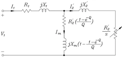
equivalent circuit model proposed by Duncan is employed [13]. The per-phase equivalent circuit model of SLIM is shown in Fig. 2. In this figure,R1 is the per–phase resist-ance of the primary calculated as:
) /( ) (
2
1 N Ws lec wAw
R = + σ (1)
In the above equation, σw is the conductivity of the
conductor used in the primary winding, lec is the end
connection length, Ws is the primary width, N is the per-phase number of turns of the primary winding and
w
A is the cross-sectional area of the conductor.
Figure 1: Structure of single-sided linear induction motor
Figure 2: Equivalent circuit of single-sided linear induction motor
The primary leakage reactance is given by [25], [26]:
p N l q W p
X s ) d) s eec] /
2 3 1 ( [(
2 0 1 2
1= µω λ + +λ +λ
(2)
where µ0 is the permeability of the vacuum, p the number of pole pairs, q the number of the slots per pole
per phase, ω1 the primary angular frequency and λs, λe and λd are the permeances of slot, the end connection and the differential, respectively.
The per-phase magnetizing reactance of the motor is given by [25]:
) /( 6 0 1 se w2 2 2 ei
m W k N pg
X = µ ω τ π (3)
where kw is the winding factor, τ is the pole pitch and
se
W and gei are the equivalent primary width and the effective air-gap length, respectively, and are calculated by the following equations:
m s
se W g
W = + (4)
tm m s l c
ei k k k g k
g = (1+ ) / (5)
In the above equation, gm=g+d is the magnetic
air-gap in which g is the air-gap length and d is the
secondary aluminum sheet thickness. kl is the air-gap
leakage factor, kc the Carter's coefficient, ktm the magnetizing reactance factor due to the edge effect, and
s
k is the secondary iron saturation factor which is calculated as [25]:
1 2
0( / ) ( )−
= i i m c
s g k
k µ τ π µδ (6)
] / 2
) / (
1 Re[
1 2
tri i i i
k s f
j π µ σ
τ π δ
+
= (7)
1 )] 2 tanh( ) 2 ( 1
[ − −
=
τ π π
τ se
se tri
W W
k (8)
In the above equations, δi is the depth of the field penetration in the secondary back-iron, s is the motor slip, σi is the conductivity of the secondary back-iron
which is reduced by the factor ktri because of the edge
effect, and µi is the secondary back-iron permeability
which should be calculated using an iterative algorithm. In this paper, the iterative algorithm proposed in [27] was employed.
For the calculation of the secondary resistance, the conductivity of the secondary sheet should be modified. The effective conductivity of the secondary sheet, σe is
given by [25]:
sk e σ/k
σ = (9)
in which
] ) / 2 cos( ) / 2 cosh(
) / 2 sin( ) / 2 sinh( [ 2
s s
s s
s sk
d d
d d
d k
δ δ
δ δ
δ −
+
= (10)
where δs is the depth of field penetration in the
secondary sheet which can be calculated by:
2 / 1 1 0
2 ]
) ( 2 1
[ + −
= µ π σ
τ π
δs fs (11)
In the above equation, f1 is the primary supply frequency, τ is the motor pole pitch, σ is the conducti-vity of the secondary sheet which is reduced by the factor
sk
k because of the skin effect due to finite plate thickness of the secondary. Besides the skin effect, the edge effect reduces the secondary conductivity by the factor ktr. If
this factor and contribution of the secondary back-iron in conduction of the secondary current are taken into account, the effective conductivity is modified to:
d k k
k tri
i i
tr sk ei
δ σ σ
σ = + (12)
The primary referred secondary resistance is defined as [28]:
ei
m G
X
where Gei is the modified goodness factor of the motor which is given by [25]:
) /( 2 0 1 2 ei ei
ei f d g
G = µ τ σ π (14)
In secondary sheet linear induction motors, the secondary reactance can be neglected [29] leading to
0 2≈ ′
X . Also, due to low value of the flux density in the
air-gap, the core loss is negligible; so, Rc ≈0. In Fig. 2,
Q is normalized motor length. The value of Q is obtained by the following equation [13]:
r m s V L L R L Q ) ( 2 2 ′ + ′ = (15)
In which, Ls is the primary length, Vr the motor
speed, Lm the magnetizing inductance, and L2′ is the secondary leakage inductance which is zero for secondary sheet motors.
Air-gap flux density is given by [25]:
] ) ( 1
/[ 2
0 m e e
g J g sG
B =µ τ π + (16)
where, Jm is the amplitude of the equivalent current
sheet which is calculated as follows [25]:
) /( 2
3 k NI1 πτ
Jm= w (17)
Using (27), the tooth flux density is obtained as:
t s g
t B w
B = τ / (18)
Referring to Fig. 2 and doing some mathematical calculations, the following equations for efficiency, power factor, output thrust and normal force are derived:
1 2 1 1 2 1 3 2 ) 1 ( 3 ) 1 ( 2 R I f F I R s s f F x m m x + − + − = τ τ η (19) 1 1 1 2 1 1 3 3 2 cos V I R I f
Fx +
= τ ϕ (20) ] ) / ( [ 2 3 2 1 2 2 2 1 2 1 2 2 1 m m m m xo X R s R X R f s R I F + + ′ + ′ = τ (21) 2 2 2 0 2 2 0 0 ) / ( cosh ) ( ) / ( sinh ) ( 1 4 m ei s ei ei s ei s s J g sV d g sV d W L Fy τ π µ σ τ π µ σ µ + − ⋅ = (22)
In the above equations, Rm is the magnetizing branch resistance in Duncan model which represents the power loss due to the end effect and Xm1 is the modified magnetizing reactance considering end effect calculated by the following equations:
2[1 Q] /
m
R =R′ −e− Q (23)
1 (1 [1 Q] / )
m m
X =X − −e− Q (24)
3. THE SLIM DESIGN
In this section, in order to design SLIM, the calculation
of the pole pitch, slot pitch, primary length, tooth and slot width are presented. The pole pitch of the motor is calculated using the following equation:
) 2 /( f1
Vs
=
τ (25)
where f1 is the input frequency and Vs is the synchronous speed. So, the slot pitch is obtained as:
) 3 /( q s τ
τ = (26)
in which q is the number of slots per pole per phase. The slot width is calculated as follows:
s s swsp
w =( )τ (27)
In the above equation, swsp is the slot width to the slot pitch ratio. It is usually chosen as a design constraint in the range of 0.4-0.7. The tooth width and the length of the primary are calculated as:
s s
t w
w =τ − (28)
τ = p
Ls 2 (29)
where p is the number of pole pairs. The primary slot
depth can be simply calculated by the following equation (see Fig. 1):
s s
s A w
h = / (30)
where As is the cross-sectional area of the primary slot which is given by:
fill w c s F A n
A = (31)
In the above equation, Ffill is fill factor of the slot and
c
n is the number of conductors per slot which is equal to:
pq N
nc = / (32)
where N is the number of turns per phase. Number of turns per coil, ncoil can be calculated using nc. For
single-layer winding nc =ncoil, and for double-layer
winding nc=2ncoil. The cross-sectional area of the
conductor of the winding is calculated by:
1 1/J
I
Aw= (33)
where I1 is primary input current and J1 is primary current density.
Using (13), (14), (23) and (24) in (21), the required MMF in order to produce the desired output thrust is obtained as: 2 2 2 2 1 1 1 1 2 2 ) / ( 3 2 m m m m X R X R R R xo K K K K s K K F f s NI MMF + + + = = ′ ′ τ (34) where the following equations are used:
2 2 K 2N
R′ = R′ (35)
2 N K R m R
m = (36)
2 1 K 1N
X
m X
m = (37)
following equation holds for the per-phase number of turns of the primary:
1 2 1 K N I
V = z (38)
where Z =KzN2 is the per-phase input impedance of the motor, in which constant KZ is equal to:
) / ( )
( 2
1 1
1 jK K jK K s
K
Kz = R + X + Rm+ Xm R′
(39) By calculation of the number of turns using (38), the calculation of the equivalent circuit parameters and other motor outputs are straightforward.
4. FREQUENCY EFFECTS
As seen in (25), changing the input frequency changes the synchronous speed (consequently the motor speed in constant slip) and/or pole pitch of the motor (motor length). On the one hand, we can study the effect of the input frequency changes on the motor dimensions and outputs in the design process; on the other hand, we can investigate the effect of the frequency effects on the performance of the SLIM for a designed motor with constant dimensions.
A. Design process
In designing a SLIM with constant speed, choosing the length of the motor depends on the value of the input frequency. Increasing the input frequency leads to a motor with short length. So, in this subsection, the effect of variation of the input frequency on the dimensions and the outputs of the motor are investigated in the design process. In these investigations, the motor is designed to produce (1000±100)N output thrust in the motor speed
of Vr =15m/s. The input phase voltage, number of pole
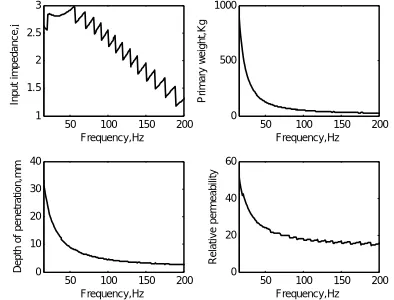
pairs and the motor slip are 220V, 2 and 0.5, respectively. Fig. 3 shows the simulation results of the motor by changing the input frequency in the design process. As it is seen in the figure, by increasing the frequency, the number of turns per phase decreases while the input current increases (except in low frequencies). The required MMF to produce constant output thrust monotonically decreases as the input frequency increases. Also, increasing frequency causes the length of the motor to decrease. It is seen that there are some jumps on the curves in Fig. 3. These jumps are because of rounding the number of turns per coil to the nearest integer in the design process. Fig. 4 shows the variation of the input impedance, the primary weight, the depth of field penetration in the secondary back-iron and its relative permeability. As seen in this figure, increasing frequency decreases the input impedance. At first, it seemed that by increasing the frequency, the input impedance would decrease. However, decreasing the input impedance is because of decreasing the number of turns per phase and accordingly decreasing the equivalent circuit parameters. Fig. 4 also shows that the primary weight decreases as the
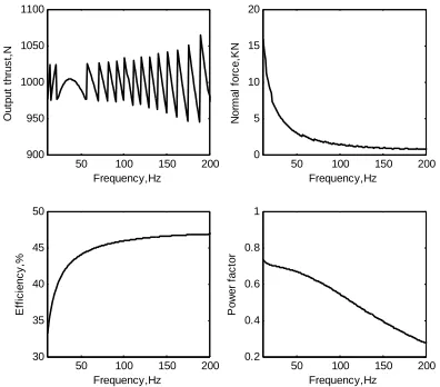
input frequency is increased. Also, increasing the input frequency causes the depth of the field penetration into the back-iron to decrease and consequently lead to reduction of relative permeability of the back-iron. The relative permeability in the figure is obtained by the iterative algorithm presented in [27]. The magnetizing curve for the sample iron used as back-iron in the design illustrated in Fig. 5 has been derived through experiment. Fig. 6 shows outputs of the SLIM versus input frequency during the design process. It is seen that increasing the frequency increases the efficiency and decreases both the power factor and the normal force while the motor produces an output thrust of (1000±100)N . Increasing the efficiency by increasing the input frequency is because of decreasing the primary resistance due to decreasing the number of turns per phase and also increasing the cross-section of the conductor with primary current density in the design process.
50 100 150 200 20
40 60 80 100 120
Frequency,Hz
Num
b
e
r of
t
u
rn
s
per phas
e
50 100 150 200 50
100 150 200
Frequency,Hz
Input
c
u
rr
ent
,A
50 100 150 200 6000
8000 10000 12000
Frequency,Hz
R
equ
ir
ed M
M
F
,A
.T
50 100 150 200 0
2 4 6 8
Frequency,Hz
M
o
to
r l
e
ngt
h
,m
Figure 3: Frequency effects on different parameters of the SLIM in design process
50 100 150 200 1
1.5 2 2.5 3
Frequency,Hz
In
p
u
t i
m
pe
danc
e,Ω
50 100 150 200 0
500 1000
Frequency,Hz
P
rima
ry
w
e
ig
h
t,
K
g
50 100 150 200 0
10 20 30 40
Frequency,Hz
D
ept
h o
f p
enet
ra
ti
on,
m
m
50 100 150 200 0
20 40 60
Frequency,Hz
R
e
la
ti
v
e
p
e
rm
e
a
b
ilit
y
0 1 2 3
x 104 0
0.5 1 1.5 2 2.5
H, A.Turn/m
B,
T
e
s
la
Figure 5: Back-iron magnetizing curve derived by experiment
50 100 150 200 0
5 10 15 20
Frequency,Hz
No
rm
a
l f
o
rc
e
,K
N
50 100 150 200 30
35 40 45 50
Frequency,Hz
E
ffi
ci
e
n
c
y,
%
50 100 150 200 0.2
0.4 0.6 0.8 1
Frequency,Hz
Po
w
e
r fa
c
to
r
50 100 150 200 900
950 1000 1050 1100
Frequency,Hz
O
u
tp
u
t th
ru
s
t,N
Figure 6: Frequency effects on different parameters of the SLIM in design process
B. Designed motor with constant parameters
In this section, the effect of the input frequency on the performance of the designed SLIM with constant parameters is investigated. The specifications of the SLIM are shown in Table I. As mentioned in the previous sections, the frequency influences the depth of the field penetration and saturation level of the secondary back-iron. For the designed SLIM, increasing the input frequency increases the input impedance and accordingly decreases the input current and the air-gap flux density. This results into a reduction of the output thrust. In order to approximately maintain the input current and the air-gap flux density constant, the input voltage is increased by increasing the frequency. So, V1/f1 is kept constant in
these investigations. In Fig. 7, the depth of the field penetration in back-iron and its relative permeability are illustrated. It is easily observed that by increasing the frequency, the depth of the field penetration and the relative permeability of the secondary back-iron are decreased. The reduction of the relative permeability is because of increasing the flux density in limited thickness of the iron due to decreasing the depth of penetration. The magnetizing curve of Fig. 5 is used in this investigation for back-iron. Fig. 8 shows outputs of the SLIM versus
input frequency. Because of the different behavior of the normal force in low and high frequencies, the curves are plotted up to frequency of 500Hz. It is seen that increasing the frequency, on one hand, increases the efficiency; on the other hand, it decreases the normal force while both the output thrust and the power factor increase in small frequency ranges and reach a maximum values and eventually decrease. As seen in the figure, the normal force becomes negative for the frequencies higher than 227Hz. It means that in this frequency range, the repulsive normal force is larger than the attractive one. This phenomenon is because of the reaction of the secondary conductor sheet. For further clarity, the attractive and repulsive normal forces are separately shown in Fig. 9. It is observed that by increasing the frequency the attractive force decreases while the absolute value of the repulsive force increases. The reason for decreasing the attractive force is that by increasing the frequency and also the input voltage (V/f constant), although the value of the amplitude of the current sheet Jm
increases (due to increasing the input current, see (17)), the value of the effective air-gap (gei) and synchronous
speed (Vs) also increase and cause the attractive normal
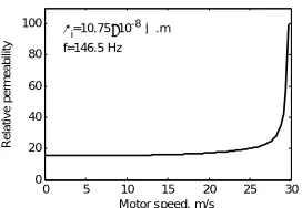
force to decrease (see (22)). The absolute value of the repulsive normal force is increased because the induced eddy currents in both the secondary sheet and the back-iron increase as the input frequency increases. Fig. 10 illustrates the depth of the field penetration and relative permeability of the secondary back-iron versus frequency in different back-iron resistivities. The figure shows that by increasing the back-iron resistivity, the depth of field penetration is increased as expected from (7). Also increasing the resisitivity of the back-iron increases the permeability of the iron, and accordingly decreases its reluctance. In Fig. 11, the relative permeability of the back-iron versus motor speed is illustrated for a constant input frequency. As seen in this figure, in low speeds, the frequency in the secondary circuit of the SLIM is high; hence, the value of the relative permeability is low. As the speed increases, the frequency in the secondary circuit of the motor decreases and causes the relative permeability to increase.
TABLE I
THE SLIMSPECIFICATIONS
Specification values Primary current density (A/mm2
) 6 Primary width (mm) 130
Secondary sheet thickness (mm) 2.0 Air gap length (mm) 5.1
Slip 0.5 Number of pole pairs 2
Number of slots/pole/phase 3 Number of turns/phase 72
Motor length, Ls (m) 0.4138
50 100 150 200 2
3 4 5 6
Frequency,Hz
D
ept
h of
penet
ra
ti
on,
m
m
50 100 150 200 0
50 100
Frequency,Hz
R
e
la
ti
v
e
p
e
rme
a
b
ilit
y
Figure 7: Frequency effects on the depth of the field penetration and back-iron permeability of the designed SLIM
100 200 300 400 500 0
500 1000 1500
Frequency,Hz
Out
put
t
h
ru
s
t,
N
100 200 300 400 500 -2000
0 2000 4000
Frequency,Hz
No
rm
a
l f
o
rc
e
,N
100 200 300 400 500 20
30 40 50
Frequency,Hz
E
ff
ici
e
n
cy,
%
100 200 300 400 500 0.2
0.3 0.4 0.5
Frequency,Hz
Po
w
e
r fa
c
to
r
Figure 8: Frequency effects on different outputs of the designed SLIM with constant dimensions
100 200 300 400 500 0
1000 2000 3000 4000
Frequency,Hz
A
tt
rac
ti
v
e
norm
a
l
fo
rc
e,
N
100 200 300 400 500 -2000
-1500 -1000 -500 0
Frequency,Hz
R
e
p
u
ls
iv
e norm
a
l
fo
rc
e,
N
Figure 9: Frequency effects on the attractive and repulsive normal force
50 100 150 200 2
4 6 8 10
Frequency,Hz
D
e
pt
h of
pene
tr
a
ti
o
n
,m
m
50 100 150 200 0
50 100 150 200 250 300 350
Frequency,Hz
R
e
la
ti
v
e
p
e
rm
e
a
b
il
it
y
ρi=10.75×10 -8Ω
.m
ρi=2×10.75×10 -8Ω.m ρi=5×10.75×10
-8Ω.m ρi=10.75×10
-8Ω.m ρi=2×10.75×10
-8Ω.m ρi=5×10.75×10
-8Ω.m
Figure 10: Frequency effects on different parameters of the designed SLIM with constant dimensions
0 5 10 15 20 25 30 0
20 40 60 80 100
Motor speed, m/s
R
e
la
ti
v
e
p
e
rm
e
a
b
ilit
y
ρi=10.75×10⁻⁸Ω.m f=146.5 Hz
Figure 11: Relative permeability of the back-iron versus motor speed
5. FINITE ELEMENT ANALYSIS
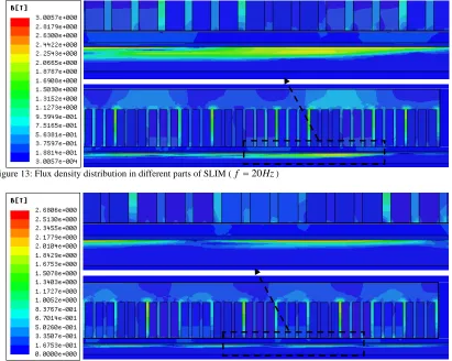
In this section, 2-D time-stepping finite element method (FEM) is employed to confirm the analytical results. The SLIM given in Table I is used in FEM simulations. In Fig. 12, the flux paths in different parts of the SLIM are depicted. The input frequency of the motor is 20Hz. In order to investigate the effect of the frequency on the depth of the field penetration and the secondary back-iron, the simulations are done with input frequency of 20 and 200Hz with constant input current. With the input current being constant, only the effects of the input frequency changes are investigated. Fig. 13 shows the flux density distribution results for f=20Hz, while in Fig. 14, those of the flux density distribution for f=200Hz are shown. The magnetizing curve shown in Fig. 5 is used for the back-iron. As seen in Figs. 13 and 14, by increasing the input frequency, the depth of the field penetration is reduced and the flux can only penetrate into a limited thickness of the secondary back-iron. Also, the flux density is increased in these regions. To compare the analytical results with those of the FEM, the simulations have been done in different input frequencies with a constant input voltage of 220 V. The efficiency, the power factor, the normal force and the output thrust are calculated using the FEM. The analytical calculation results are compared with the FEM results in Table II. It is easily seen that as input frequency increases the efficiency increases while the power factor, the normal force and the output thrust decrease. The reason for different behaviors of the output thrust and the power factor in this table and those given in figure 8 is the applied constant input voltage in the FEM simulations. As stated before, in deriving the results of figure 8, the input voltage is increased as the input frequency increases (V1/f1
constant). However, it is seen that the results of the two methods are close enough to each other confirming the analytical calculations.
Figure 12: Flux paths in the moving SLIM (f =20Hz)
6. CONCLUSION
Figure 13: Flux density distribution in different parts of SLIM (f =20Hz)
Figure 14: Flux density distribution in different parts of SLIM (f =200Hz)
TABLE II
THE CALCULATION AND FEM RESULTS
Output thrust (KN) Normal force (KN)
Power factor Efficiency (%)
32.01 137.18
0.5252 37.59
Analytical
32.05 136.21
0.5447 35.71
FEM f=20Hz
7.32 17.91
0.5211 43.20
Analytical
7.35 18.01
0.5409 41.42
FEM f=50Hz
2.18 2.89
0.4898 45.38
Analytical
2.20 2.81
0.5093 44.04
FEM f=100Hz
0.57 0.21
0.4192 46.63
Analytical
0.58 0.20
0.4302 44.91
FEM f=200Hz
0.073 -0.069
0.2824 47.52
Analytical
0.069 -0.060
0.3101 45.97
FEM f=500Hz
the normal force and the output thrust of the SLIM have been derived considering the longitudinal end effect, iron saturation, transverse edge effect, and skin effect. The results show that increasing the frequency decreases the active and usable thickness of the secondary back-iron. Hence, for high frequency SLIMs, the thickness of the secondary back-iron can be limited to the depth of the field penetration in the iron. It should be emphasized that
7. REFERENCES
[1] S. Nonaka and T. Higuchi, “Elements of linear induction motor design for urban transit”, IEEE Trans. Magn.,Vol. 23, No. 5, pp. 3002-3004 , September 1989.
[2] S. Yoon, J. Hur and D. Hyun, "A method of optimal design of single-sided linear induction motor for transit", IEEE Trans. Magn.,Vol. 33, No. 5, pp. 4215-4217, September 1997.
[3] W. Xu, J. Zhu, L, Tan, Y. Guo, S, Wang, and Y. Wang, “Optimal design of a linear induction motor applied in transportation”, IEEE Int. Conf. on Ind. Tech., pp. 1-6, 2009.
[4] D. Yumei and J. Nenggiang, “Research on characteristics of single-sided linear induction motors for urban transit”, IEEE Int. Con. on Elect. Machines and Systems, ICEMS, pp.: 1-4, 2009. [5] S. Osawa, M. Wada, M. Karita, D. Ebihara and T. Yokoi,
“Light-weight type linear induction motor and its characteristics”, IEEE Trans. Magn.,Vol. 28, No. 4, pp. 3003–3005, September 1992. [6] M. Kitamura, N. Hino, H. Nihei and M. Ito, “A direct search shape
optimization based on complex expressions of 2-dimentional magnetic fields and forces”, IEEE Trans. Magn.,Vol. 34, No. 5, pp. 2845–2848, September 1998.
[7] B. Laporte, N. Takorabet and G. Vinsard , “An approach to optimize winding design in linear induction motors”, IEEE Trans. Magn.,Vol. 33, No. 2, pp. 1844–1847, March 1997.
[8] T. Mishima, M. Hiraoka and T. Nomura, “A study of the optimum stator winding arrangement of LIM in maglev systems”, IEEE Int. Conf. on Electric Machines Drives, IEMDC, pp. 1238–1242, May 2005.
[9] A. Hassanpour Isfahani, H. Lesani and B. M. Ebrahimi, “Design optimization of linear induction motor for improved efficiency and power factor”, IEEE Int. Conf. on Electric Machines Drives, IEMDC, pp. 988–991, May 2007.
[10] A. Hassanpour Isfahani, B. M. Ebrahimi, and H. Lesani, “Design optimization of a low-speed single-sided linear induction motor for improved efficiency and power factor”, IEEE Trans. Magn., Vol. 44, No. 2, pp. 266–272, February 2008.
[11] C. Lucas, Z. Nasiri G. and F. Tootoonchian, "Application of an imperialist competitive algorithm to design of linear induction motor", Energy Conversion and Management, Vol. 51, pp. 1407-1411, 2010.
[12] D. H. Im, S. C. Park, and J. W. Im, “Design of single-sided linear induction motor using the finite element method and SUMT”, IEEE Trans. Magn.,Vol. 29, No. 2, pp. 1762-1766, March 1993. [13] J. Duncan, "Linear Induction motor-equivalent circuit model", IEE
Proc. on Electric Power Appl., Vol. 130, No. 1, pp. 51-57, 1983. [14] S. Nonaka, "Investigation of equivalent circuit quantities and
equations for calculation of characteristics of single-sided linear induction motors (LIM)", Elec. Eng. in Japan, Vol. 117, No. 2, pp. 107-121, 1996.
[15] S. Nonaka, "Investigation of equations for calculation of secondary resistance and secondary leakage reactance of
single-sided linear induction motors", Elec. Eng. in Japan, Vol. 122, No. 1, pp. 60-67, 1998.
[16] W. Xu, J. G. Zhu, Y. Zhang, Y. Li, Y. Wang, and Y. Guo, “An Improved equivalent circuit model of a single-sided linear induction motor”, IEEE Trans on Vehicular Tech., Vol. 59, No. 5, pp.:2277-2289, June 2010.
[17] W. Xu, J. G. Zhu, Y. Zhang, Z. Li, Y. Li, Y. Wang, Y. Guo, and W. Li, “Equivalent circuits for single-sided linear induction motors”, IEEE Trans on Ind. Appl., Vol. 46, No. 6, pp.:2410-2423, Nov./Dec. 2010.
[18] S. G. Lee, H. Lee, S. Ham, C. Jin, H. Park, and J. Lee, “Influence of the construction of secondary reaction plate on the transverse edge effect in linear induction motor”, IEEE Trans. Magn.,Vol. 45, No. 6, pp. 2815-2818, June 2009.
[19] J. F. Gieras, G. E. Dawson, A. R. Easthan, “A new longitudinal end effect factor for linear induction motor”, IEEE Trans. Energy Convers., Vol. 2, No. 1, pp.: 152-159, March 1987.
[20] R. C. Creppe, J. A. C. Ulson and J. F. Rodrigues, “Influence of design parameters on linear induction motor end effect”, IEEE Trans. Energy Convers., Vol. 23, No. 2, pp.:358-362, June 2008. [21] J. Lu and W. Ma., “Research on end effect of linear induction
machine for high-speed industrial transportation”, IEEE Trans on Plasma Sci., Vol. 39, No. 1, pp.: 116-120, January 2011. [22] T. Yang, L. Zhou, and L. Li, “Influence of design parameters on
end effect in long primary double-sided linear induction motor”, IEEE Trans on Plasma Sci.,Vol. 39, No. 1, pp.:192-197, January 2011.
[23] A. S. Gercek and V. M. Karsli, “Performance prediction of the single-sided linear induction motors for transportation considers longitudinal end effect by using analytical method”, Contemporary Engineering science, Vol. 2, No. 2, pp: 95-104, 2009.
[24] A. Z. Bazghaleh, M. R. Naghashan and M. R. Meshkatoddini, “Optimum design of single-sided linear induction motors for improved motor performance”, IEEE Trans. Magn.,Vol. 46, No. 11, pp. 3939–3947, November 2010.
[25] I. Boldea, S. A. Nasar, Linear motion electromagnetic devices, Taylor & Francis, New York 2001.
[26] S. A. Nasar and I. Boldea, Linear electric motors, Prentice-Hall, Inc., Englewood Cliffs, New Jersey, 1987.
[27] M. Mirsalim, A. Doroudi and J. S. Moghani, “Obtaining the operating characteristics of linear induction motors: a new approach”, IEEE Trans. Magn.,Vol. 38, No. 2, pp. 1365–1370, March 2002.
[28] E. R. Laithwaite, Induction machines for special purposes, George Newnes Limited, London 1996.