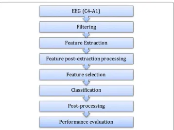
A knowledge discovery methodology
from EEG data for cyclic alternating pattern
detection
Fátima Machado
1, Francisco Sales
2, Clara Santos
3, António Dourado
1and C. A. Teixeira
1*Abstract
Background: Detection and quantification of cyclic alternating patterns (CAP) components has the potential to serve as a disease bio-marker. Few methods exist to discriminate all the different CAP components, they do not present appropriate sensi-tivities, and often they are evaluated based on accuracy (AC) that is not an appropriate measure for imbalanced datasets.
Methods: We describe a knowledge discovery methodology in data (KDD) aiming the development of automatic CAP scoring approaches. Automatic CAP scoring was faced from two perspectives: the binary distinction between A-phases and B-phases, and also for multi-class classification of the different CAP components. The most important KDD stages are: extraction of 55 features, feature ranking/transformation, and clas-sification. Classification is performed by (i) support vector machine (SVM), (ii) k-nearest neighbors (k-NN), and (iii) discriminant analysis. We report the weighted accuracy (WAC) that accounts for class imbalance.
Results: The study includes 30 subjects from the CAP Sleep Database of Physionet. The best alternative for the discrimination of the different A-phase subtypes involved feature ranking by the minimum redundancy maximum relevance algorithm (mRMR) and classification by SVM, with a WAC of 51%. Concerning the binary discrimination between A-phases and B-phases, k-NN with mRMR ranking achieved the best WAC of 80%.
Conclusions: We describe a KDD that, to the best of our knowledge, was for the first time applied to CAP scoring. In particular, the fully discrimination of the three different A-phases subtypes is a new perspective, since past works tried multi-class approaches but based on grouping of different sub-types. We also considered the weighted accuracy, in addition to simple accuracy, resulting in a more trustworthy performance assessment. Globally, better subtype sensitivities than other published approaches were achieved.
Keywords: Cyclic alternating pattern, A-phase detection, EEG processing, Knowledge discovery in data
Open Access
© The Author(s) 2018. This article is distributed under the terms of the Creative Commons Attribution 4.0 International License (http://creat iveco mmons .org/licen ses/by/4.0/), which permits unrestricted use, distribution, and reproduction in any medium, provided you give appropriate credit to the original author(s) and the source, provide a link to the Creative Commons license, and indicate if changes were made. The Creative Commons Public Domain Dedication waiver (http://creat iveco mmons .org/publi cdoma in/zero/1.0/) applies to the data made available in this article, unless otherwise stated.
RESEARCH
*Correspondence: [email protected] 1 CISUC-Centro de Informática e Sistemas da Universidade de Coimbra, Departamento de Engenharia Informática, Faculdade de Ciências e Tecnologia, Universidade de Coimbra, 3030-290 Coimbra, Portugal
Background
A cyclic alternating pattern (CAP) sequence is composed by a succession of CAP cycles, each one composed by two types of phases: The A-phases and the B-phases. The A-phases in lighter stages of comas are closely related to hyperventilation, restless, increase of pulse rate, and can be associated with increase in muscle activity. In con-trast, autonomic and muscular activities are attenuated during the B-phases. Investiga-tions discovered also that CAP is a physiologic component of non-rapid eye movement (NREM) sleep stages and do not occur, under normal conditions, in rapid eye movement (REM) [1, 2]. CAP sequences tend to appear associated with some dynamic sleep events like a change in sleep stages, falling asleep, or arousal without awaking [3]. However, some pathological conditions generate CAP sequences in REM, therefore it has potential to be used as a prognostic element of such diseases. Higher CAP rates are present in some types of insomniac patients [4], epilepsies [5], among other disorders. Thus, CAP quantification could be used as diseases biomarker, for example for seizure prediction [6].
The CAP definition and scoring rules are described in [7]. CAP is defined there as “a periodic EEG activity of NREM sleep characterized by sequences of transient electrocor-tical events, that are distinct from the background electroencephalogram (EEG) activity and reoccur at up to 1-minute intervals”. An A-phase is considered as a transient phe-nomenon translated by an increase in amplitude and/or frequency which is clearly dis-tinguishable from background activity, i.e. from the B-phase, and is associated to a brain activation, including cortical arousal. For this reason, an A-phase is a potential trigger of somatomotor activities. Each phase can have a duration between 2 and 60 s. The mean duration of CAP sequences in young adults is two and half minutes, which contains in average six CAP cycles [1]. If an A-phase is not preceded and succeeded by another A-phase in 60 s, it is considered an isolated A-phase and defined to not belonging to a CAP cycle. To form a CAP sequence, at least two consecutive CAP cycles are required. An A-phase can be composed by high-voltage slow waves which are manifestations of EEG synchrony, by low-amplitude fast rhythms that are evidence of the EEG desyn-chrony and be associated with typical waveforms (for example K-complexes). Depending on the associated waveforms and on the percentage of each wave type, a given A-phase is classified into three different subtypes:
• Subtype A1: It is composed by high-voltage slow waves. This subtype can be classi-fied by an increase in amplitude of at least a third of the normal background activity. The synchronized EEG pattern must occupy more than 80% of the epoch to be clas-sified as A1. The associated waveforms with this subtype are bursts, and K-complex sequences.
• Subtype A2: This subtype has elements from subtypes A1 and A3, and, therefore, it is composed by a mixture of fast and slow rhythms. The elements from the subtype A1 must occupy between 50 and 80% of the length of an entire A-phase. In this subtype, the typical waveforms are polyphasic bursts.
To mention also that the A-phases subtypes present different signatures in the con-ventional EEG frequency bands: delta ( δ= [1, 4] Hz), theta (θ = [4, 8] Hz), alpha (α = [8,
13] Hz), sigma (σ = [13, 16] Hz) and beta (β = [16, 35] Hz) [8].
Different algorithms have been proposed in the last years for automatic scoring of A-phases and B-phases. Barcaro et al. proposed a detection method for A-phases [9–11], more precisely in [10, 11] these authors considered only three classes: B, A1 and A2/A3 phases. The association of subtypes A2 and A3 was due to their similarity, as reported in the literature. The rationale of the methodology was the same in both papers [10, 11]: an amplitude feature was computed for each of the conventional frequency bands and then compared with a threshold. When one of the five features crossed the threshold a tenta-tive A-phase detection was performed. The type assigned to the A-phases detected (A1 or A2/A3) depended on which features crossed the threshold. The best reported results were the ones proposed with the methodology presented in [11], which had a correct-ness of 83.5% for the binary discrimination between A-phases and B-phases, and 73.7% for the multi-class distinction between A1, A2/A3 subtypes.
A model based on feedback loops that simulates the EEG activity was proposed by [12]. This methodology was used to detect K-complexes and vertex waves and detected CAP sequences by considering four rhythm generators, which corresponded to different frequency bands (δ, α, θ and σ). The results obtained with this algorithm pointed for a mean sensitivity of 90% [12].
A method based on wavelets and genetic algorithm was proposed in [13] to identify the A-phases independently of the subtype. Basically, the signal was decomposed into five signals corresponding to the different frequency bands, using the discrete wave-let transform. A feature based on amplitude was computed for each decomposed sig-nal. The A-phases were detected comparing the features to a threshold. The accuracy reported was 79%.
Stam and van Dijk [14] published a study that defined the synchronization likelihood (SL) between two EEG channels and proposed a method to calculate this value. This measurement was applied for A1 detection [15], where the signal was filtered between 0.25 and 2.5 Hz. They concluded that during sleep the levels of SL in this frequency range had significant fluctuations with CAP occurrence. This feature presented a good performance in distinguishing the A1 subtype from the background [16]. Although this was only true for NREM stage 2. For the others sleep stages this feature cannot distin-guish A1 or the other subtypes [15, 16].
However, the approaches previously reported did not present a good performance to score correctly the microstructure without a posteriori technician revision. Moreover, good results were only obtained for the distinction between A-phases and B-phases, and not for the multi-class discrimination between all the different subtypes. Another draw-back was the consideration of simple accuracy that lead to an overestimation of the per-formance in imbalanced datasets, which is the case of A-phase scoring.
Here, we describe a knowledge discovery methodology in data (KDD) that is for the first time applied to CAP scoring. The KDD encompasses: the extraction of multiple EEG features, different pre-processing options, and different pattern recognition tech-niques. The KDD aims to inspect about proper processing alternatives for the binary distinction between A-phases and B-phases, and also for multi-class classification of the different CAP components, i.e. the three A-phase subtypes as well as the B-phases. The fully discrimination of the three different A-phases subtypes is a new perspective, since past works tried multi-class approaches but based on grouping of different sub-types, as for example A2 and A3. We also considered the weighted accuracy, in addition to simple accuracy, resulting in a more trustworthy performance assessment. The next sec-tion describes the methods used, the database and data characteristics. “Results” section describes the classification performance achieved for the different options considered. Insights about results and future directions are given in “Discussion” and “Conclusion” sections.
Methods
Database
The study was carried out on 30 subjects with nocturnal frontal lobe epilepsy, 14 females and 16 males, with ages between 14 and 67 years old (mean = 31.03 ± 11.64). The data-set is available from the CAP Sleep Database [18], that comprises several one-night polysomnographic recordings from different patients with different pathologies, and has been used in several studies in the past [10, 11, 13, 17, 19]. The recordings were acquired at the Sleep Disorders Center of the Ospedale Maggiore of Parma, Italy. The polysom-nographic data includes at least three EEG channels (F3 or F4, C3 or C4 and O1 or O2, referred to electrodes placed in the earlobes, labeled as A1 or A2), two EOG channels, three electromyography signals (EMG), respiration signals and the ECG. The sampling rates for the recordings vary from 128 to 512 Hz, depending on the patient.
The macrostructure and microstructure scoring were annotated by neurophysiolo-gists and supplied together with the raw EEG data. The macrostructure was annotated according to the R&K rules [20], while CAP was detected in agreement with Terzano reference atlas [7].
Knowledge detection methodology in data
Filtering
The original signal was filtered to obtain its components in six frequency bands, i.e. in the band 0.3–35 Hz [originating a signal called in this work as the broadband signal (BB)], and in the five conventional frequency sub-bands. The filter of the signal between 0.3 and 35 Hz was chosen to be in agreement with the usual practice in clinics [21]. The five conventional frequency bands considered were: delta (δ: 0.3–4 Hz), theta (θ: 4–8 Hz), alpha (α: 8–13 Hz), sigma (σ: 13–16 Hz) and beta (β: 16–35 Hz), that will be designated by conventional frequency bands [8] along this article.
The EEG signal was filtered using a third-order band-pass Butterworth filter [22] and was chosen due to its flat and without ripples frequency response in both pass- and stop-bands.
Feature extraction
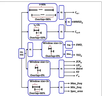
Features were extracted from EEG recordings that have a duration of a whole night of sleep (around 8 h). Each feature had a value for each second by segmenting using a slid-ing window approach. Overall, different window sizes and different degrees of super-position between consecutive windows were considered. The options for the different features are presented in Fig. 2. Also, for two features, segmentation was performed after features computation. The need to define different segmentation procedures was due to the particularities of the different features. Details on the computation of each feature will be described in the following sections.
Macro–micro structure descriptor
Macro–micro structure descriptor (MMSD) is an a-dimensional and normalized meas-urement of how the mean amplitude, C, of the EEG signal in a given frequency band ϕ(ϕ⊂ {δ,θ,α,σ,β}) ) differs, at a given time instant, from its background. The MMSD is given by [1],
This means that MMSDϕ results from the combination of two primary features Cϕ,τ and Cϕ,τ0 that were also considered in this work. In a general way, Cϕ,τ represents the mean amplitude at a given time instant, computed taking in account the past samples over an interval of size τ . If τ is long enough, it represents the background of the
sig-nal, while if it is too short it is related with instantaneous signal activity. It was reported that if τ =60s and τ0=2s , Cϕ,τ and Cϕ,τ0 are generally related to the sleep macro- and microstructure, respectively [9]. Therefore, these were the values used to compute (1)
MMSDϕ =
Cϕ,τ0−Cϕ,τ
Cϕ,τ .
MMSDϕ , Cϕ,τ0 and Cϕ,τ . Given the MMSDϕ dependence on the sleep microstructure, it has been used to classify A-phases [9–11].
One the one hand, given the selected τ value, MMSDϕ and Cϕ,τ were computed by considering a window of 60 s and a superposition between consecutive windows of 59 s (98% overlap). On the other hand, τ0 defines that Cϕ,τ0 was computed based on a window of 2 s and a superposition between consecutive windows of 1 s (50% of overlap).
Teager energy operator
The Teager energy operator (TEO) gives a non-linear measure of the instantaneous signal energy [23, 24]. In its discrete form TEO is given by [2],
where x[n] is the discrete signal sequence. This operator has been successfully used in several signal processing applications. For example, it was used in speech processing [25, 26], and feature extraction from EMG signals [27]. TEO has been referred as adequate for the identification of some EEG elements which are crucial for the CAP scoring, like sleep-spindles [28], and K-complexes [29]. TEO was computed for all the EEG signal and for all frequency bands and was applied in first place to the entire EEG time series due to its non-causal formulation. Afterwards, the TEO sequence was divided into epochs of 1 s and each one is represented by the maximum TEO value.
Zero‑crossing rate
Zero-crossing rate (ZCR) is a measure of the dominant frequency of a signal, and is obtained in the time domain by counting the number of baseline crossings in a fixed time interval [30]. The ZCR is a fast, intuitive and low complexity way to obtain infor-mation about the signal frequency in a short period of time [31, 32]. This feature has been widely used in different applications [33], in particular in the sleep staging field [30, 34]. To compute this feature a non-overlapping moving window of 1 s duration was considered.
Lempel–Ziv complexity
Lempel–Ziv complexity (LZC) is a metric used to evaluate the randomness of finite sequences proposed by Lempel and Ziv, in 1976 [35], and has been used to character-ize sleep [36, 37]. To compute the LZC complexity a numerical sequence has to be transformed into a symbolic sequence. A frequent approach is to convert the signal,
x[n], into a binary sequence, P =s[n], and comparing the signal with a threshold, Td.
The points whose value is greater than Td are converted to 1, otherwise to 0.
After-wards, a dictionary is build based on the sequences present in the signal s[n]. The size of the dictionary is proportional to the LZC. The methodology used to compute this feature is described in [38]. LZC as well as ZCR were computed for the six signals: broadband signal and five frequency bands, and using a non-overlapping moving win-dow of 1 s.
(2)
Discrete time short time Fourier transform
Discrete Fourier transform (DFT) is the simplest form of time–frequency analysis for discrete stationary signals, and is given by [3],
where N is the total the number of samples in a given signal segment, x[n] is the value of the signal at instant n and k is the discrete frequency bin (0 to N − 1).
The EEG is a non-stationary signal, with different intervals of time having different frequency contents. If the DFT is applied to the signal the evolution of frequencies with time will be lost. To overcome this, the solution is to divide the signal into pieces through the application of a window, w, and apply the DFT [39] to each one, leading to the discrete time short time Fourier transform (DTSTFT), given by [4],
The window w[n] is assumed to be non-zero only in an interval of length Nw and is referred
to as the analysis window. The sequence x[m]w[n −m] is called short section of x[m] at time
n [40]. In this work, for each window, it was obtained a spectrum and from it was extracted the frequency of maximum energy ( Max_freq ), the frequency of mean energy ( Mean_freq ) and the area under the magnitude spectrum curve ( Spec_area ). The spectrum was com-puted considering a window length of 3 s, with an overlap between windows of 2 s.
Empirical mode decomposition
In empirical mode decomposition (EMD) a given signal is decomposed in intrinsic mode functions (IMF), where each one represents an embedded characteristic oscillation on a separated time-scale. The EMD application requires a continuous signal, with the num-ber of maxima equal to the numnum-ber of minima, and also a signal with zero mean. The EMD has been used in EEG applications, for example, for classification of mental tasks [23] and in automatic sleep staging using ECG [41].
In this work EMD was computed for 12 decomposition levels, and the procedure used is available in [42]. To overcome problems with EEG segmentation EMD was applied to the entire signal and segmented afterwards by using consecutive windows of 1 s without overlap. The features derived from EMD were the average values of the different IMFs obtained for each window.
Shannon entropy
Shannon entropy (ShEnt) evaluates the randomness (complexity) of a signal by comput-ing its amplitude distribution and the probability for a given value to occur. The higher the probability for the values to happen, the less information exists on the signal, result-ing in a smaller entropy. ShEnt has been widely used in EEG processresult-ing, for example to distinguish between normal and epileptic EEG [43]. It was proved that this feature is proportional to the sleep macro and microstructure [44] and it has been applied in the (3)
X[k]=
N−1
n=0
x[n]e−j2πknN ,
(4)
X[n,k]= ∞
m=−∞
automatic sleep staging [45–48]. A non-overlapping moving window of 1 s duration was applied to the broadband signal, then the ShEnt was computed.
Fractal dimension
Fractal dimension (FD) quantifies the number of times the same sequence appears in a signal. A signal can be composed by basic building-blocks forming a pattern, the FD quantifies the number of these basic building-blocks. The algorithm proposed by Higu-chi [49] is generally used for finding FD in EEG signals.
Fractal dimension is related with sleep macro and microstructure [44] and has been used in the automatic staging of sleep patterns [45, 47]. The broadband signal was divided into epochs of 1 s length, afterwards the FD was computed for each one of them.
Variance
Variance has been used for automatic sleep staging [47] and A-phases detection [17]. The formula for variance computation, s2, is on Equation [5], where N is the number of signal samples, x[n] is the value of the n-th signal sample and x¯ the mean value of the
signal over the time interval [1,N].
Variance was computed by segmenting the broadband EEG signal with a non-overlap-ping moving window of 1 s duration.
Summary
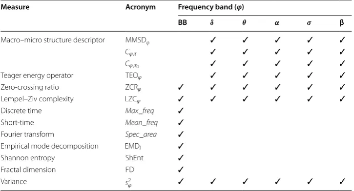
Given the different decomposition levels, and the considered frequency bands, a total of 55 features were obtained. Table 1 summarizes which features were considered and for which (5) s2= 1
N−1
N
n=1
(x[n]− ¯x)2
Table 1 Computed EEG features
BB stands for broadband EEG signal, and δ , θ , α , σ and β are the conventional frequency bands. The ϕ specifies the frequency
band considered, and the (✓) symbol indicate if a given measure was extracted for a given frequency band. Concerning
EMDl , l represents the decomposition level that in this paper can assume valued from 1 to 12
Measure Acronym Frequency band (φ)
BB δ θ α σ β
Macro–micro structure descriptor MMSDφ ✓ ✓ ✓ ✓ ✓
Cϕ,τ ✓ ✓ ✓ ✓ ✓
Cϕ,τ0 ✓ ✓ ✓ ✓ ✓
Teager energy operator TEOϕ ✓ ✓ ✓ ✓ ✓
Zero-crossing ratio ZCRϕ ✓ ✓ ✓ ✓ ✓ ✓
Lempel–Ziv complexity LZCϕ ✓ ✓ ✓ ✓ ✓ ✓
Discrete time Max_freq ✓
Short-time Mean_freq ✓
Fourier transform Spec_area ✓
Empirical mode decomposition EMDl ✓
Shannon entropy ShEnt ✓
Fractal dimension FD ✓
Variance s2
frequency band were extracted. At the end, a feature name is composed by its name con-catenated with the frequency band considered. For example, the Teager energy extracted for the EEG signal in the θ band is described by TEOθ . EMD was computed for 12 decom-position levels and is represented by EMDl , where l=1, 2,. . ., 12 , represents each level. Details about the window size used and percentage of superposition between windows are given in Fig. 2. For TEOϕ and for EMDl segmentation was performed after feature com-putation in order to comply with the TEOϕ non-causal characteristic, and to discard the windowing effect that has drastic consequences for EMDl . To mention that the window lengths and overlaps defined guaranties the sampling rate of 1 s for all the features.
Features post‑extraction processing
Firstly, all features except MMSD, TEO and EMD were smoothed using a causal mov-ing average FIR filter of order 30 [50]. These features were excluded because they detect changes in amplitude and frequency, and if the smoothing technique had been applied, important information could had been lost.
Secondly, the samples four standard deviations away from the mean were considered outliers. Their values were replaced by the median of the feature. If the frequently used value of three standard deviations would be used, the A-phases would likely be consid-ered as outliers. Therefore, the maximum distance allowed was extended. Finally, the values of each feature were normalized to be in the [0–1] range.
Feature ranking and transformation
The selection or reduction of the features used for the classification task is essential for a good performance of the classifier, on the one hand it is desired that the features should be correlated with the class labels, on the other hand they should not be redundant among themselves. Feature selection and transformation also contributes to reduce the computational cost associated with high dimensionality problems (the “curse of dimen-sionality”). So, the features must be analyzed aiming to select the best set to use in the classification step. In this work two approaches were used, one for feature selection by ranking and other for feature transformation by projection:
• Minimum redundancy maximum relevance (mRMR): This algorithm ranks the fea-tures based on two objectives: obtain the highest correlation between the selected features and class labels (maximum relevance) and reduce the redundancy between features (minimum redundancy). This technique is described in detail in references [51].
Classification
Different linear and non-linear classification methods were used in this work aiming to see for which methods and conditions a better performance was achieved. From the pre-vious steps 55 features were obtained, and each feature had a value and a class label for each second, thus we trained the models to classify the EEG signal at every second. The class labels were computed based on the original annotations provided for the raw EEG data, as described in “Database” subsection. The different classification methods consid-ered are described next.
Discriminant analysis
Discriminant analysis (DA) [53] has been used in different areas like in statistics, pattern recognition and machine learning. Considering a feature vector x of size (d×1) , and c classes ωk ( k=1, 2,. . .,c ). To find the best discrimination function,
g, the first step is to define the function type. It can be linear, g(x)=wx+w0 and in this case the classifier performs a linear discriminant analysis (LDA), or quadratic, g(x)=w0+di=1wixi+di=1
d
j=1xixjwij , and in this case a quadratic discriminant analysis (QDA) is implemented, where w is the weight vector and w0 is the bias.
The weights (w, w0 ) are computed by minimizing a cost function of the classification errors by using N examples as training data:
where tn is the n-th sample of the target vector, i.e. the label of sample xn.
In a multi-class problem with c classes, where c>2 , the discrimination procedure is to compute the c discriminant functions. The linear discriminant functions are given by gk(x)=wTkx+wk,0 . To each point assign a class ck if gk(x) assume the highest value among all the discriminant functions.
k‑Nearest neighbors (k‑NN)
k-Nearest neighbors is a non-parametric method, which means that there is no assump-tion about the underlying pattern distribuassump-tions. Unlikely the DA the k-NN does not find the best function to divide the space into regions. Instead, the training data is stored in a matrix containing the features and the labels assigned to each pattern. To label a new point, x, it is compared with the k-closest training points. The class assigned to x is the most prevalent class in these k-points [54].
Support vector machines
In its native formulation support vector machine (SVM) finds a decision hyperplane that maximizes the margin that separates the two different classes [55].
Considering the training data xi,yi
, i=1,. . .,N , ti∈ {−1, 1} , xi∈Rd , where ti are the class labels and xi the features values. Considering that the data is non-linearly
sepa-rable, the function which define the hyperplane is [7],
(6)
J(w)= 1
N N
n=1
tn−g(xn,w)
2
where w is the vector normal to the hyperplane, b
w is the hyperplane offset to the origin and ξ is a quantification of the degree of misclassification. w and b are obtained by mini-mizing [8],
due C defines the influence of ξ on the minimization criterion Ψ.
In the previous case, the boundary that separates the classes is linear. To improve clas-sification in non-linearly separable data the features space is projected into a higher dimensional space based on a Kernel projection where the linear separability principle can be applied. The most popular Kernel, which is used in this work, is the Gaussian Kernel [9],
where xj is the position of the Gaussian centre and σ the Gaussian aperture (standard
deviation).
The SVM is defined as a two-class classifier, but A-phase classification is a multi-class problem. The usual approach for multi-class SVM classification is to use a combination of several binary SVM classifiers. Different methods exist but in this work we used the one-against-all multi-class approach [56]. This method transforms the multi-class prob-lem, with c classes, into a series of c binary sub problems that can be solved by the binary SVM. The i th classifier output function ρi is trained taking the examples from ci as 1 and
the examples from all other classes as − 1. For a new example x, this method assigns x to the class associated with the largest value of ρi [56].
Post‑processing
The unique post-processing implemented was focused on the validation the A-phase duration that must be within the interval 2 s to 60 s. Thus, the number of consecutive 1 s epochs classified as A-phases were quantified. If a single epoch was classified as A-phase, or if more than 60 consecutive epochs were classified as A-phases, they were considered as background signal, i.e. as B-phases.
Performance evaluation
The Leave-one-out approach [57] was used, which is the most classical exhaustive cross validation (CV) procedure. Supposing that the data is composed by M patients, the algo-rithm will be trained M times. In each iteration, a different patient is “left out” to be the test data and the remaining ones are training data. The algorithm output for each patient is compared to the real staging by filling confusion matrices. We evaluated the algo-rithms from two perspectives: the performance on detecting A-phases from B-phases (binary problem) and the algorithms capabilities to differentiate among the different (7) ti
wTxi+b≥1−ξi t∈ −1;1
(8) Ψ (w)= 12�w�2+CN
i=1
ξi, subject to
yi
wTxi+b
≥1−ξi, i=1, ..,N,
(9)
k
xi,xj
=eγ�xi−xj�2, γ = 1
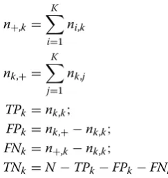
CAP subcomponents, i.e. the capability to differentiate A1, A2, A3 and B phases (multi-class problem). Thus, two confusion matrices were filled, which can be represented by the generic confusion matrix in Table 2.
For the binary problem c= {A-phase, B-phase}, while for the multi-class problem c= {B-phase, A1, A2, A3}. In Table 2 the diagonal terms nij , where i=j , correspond to
the instances where the algorithm’s output was consistent with to the real class label, i.e. the true positive patterns. The values nij , where i�=j , are the number of instances mis-classified by the algorithm, which can be considered as false positives or false negatives depending on the class under analysis.
Considering a given class k, four measurements were taken:
• True positive ( TPk ): number of instances correctly classified as class k;
• False positive ( FPk ): number of instances classified as k when in fact they belong
to other class;
• True negative ( TNk ): number of instances correctly not classified as k;
• False negatives ( FNk ): number of instances assigned to other classes when in fact
they belong to class k;
For a classification problem with K classes, these measurements can be computed from the confusion matrix as follows in [10].
To evaluate the algorithm’s three performance measures were used: sensitivity (SE), specificity (SP) and accuracy (AC), which are given by [11]:
(10)
n+,k = K
i=1 ni,k
nk,+=
K
j=1 nk,j
TPk =nk,k;
FPk =nk,+−nk,k;
FNk =n+,k−nk,k;
TNk =N−TPk−FPk−FNk
(11)
SEk =
TPk TPk+FNk
; SPk =
TNk TNk+FPk
;
AC= TNk+TPk
TNk+FPk+FNk+TPk
.
Table 2 Generic confusion matrix, where “^” indicates predictions provided by the algorithms
Predicted True
c1 c2 · · · cK
c1 n1,1 n1,2 · · · n1,K
c2 n2,1 n2,2 · · · n2,K
. .
. · · · ·
The B-phases, i.e. background epochs, were more present than the A-phases, some-times seven some-times more. Therefore, when an algorithm correctly detected most of the B-phases, even though performance was not as good as A-phases, it usually had a higher accuracy. Since the main objective was to correctly detect the A-phases, the AC might not yield a correct view of the overall performance of the algorithm. A more adequate performance measure was considered, the weighted accuracy (WAC), that takes into account the number of instances of each class. Thus, a miscomputation of B-phase instance will have lower impact on accuracy than an A-phase misclassifi-cation. The weighted accuracy is given by [12].
AC is also presented, although it provides poorer performance, to better compare the results with those reported in literature.
Results
In total, 55 features were computed. An evaluation of the performance using different num-ber of features and principal components to build a classifier was performed and the results are shown in the following sub-sections. A straightforward approach was implemented and worked as follow: (i) at start only the two more important features or principal components were considered; (ii) then we introduced the next feature/principal component in the next step; (iii) until all the features/components were considered as classifier’s input.
Multi‑class A‑phase classification mRMR
Features ranking with mRMR did not returned exactly the same result for all the patients, being an evidence of the inter-individual variability. Analyzing all the rankings sequences for each patient, the most prevalent ranking sequence was (from higher to lower importance): LZCBB , Cβ,τ , Cσ,τ , Cβ,τ0 , Cσ,τ0 , Cδ,τ , ZCRBB , Cδ,τ0 , Max_freq , Cα,τ0 , Cθ,τ , MMSD , Cθ,τ0 , Cα,τ , TEOδ , MMSD , EMD1 , s2δ , MMSDσ , EMD2 , EMD6 , MMSDα , EMD5 ,
EMD7 , MMSDβ , s2θ , MMSDσ , Spec_area , sBB2 , EMD10 , EMD4 , sβ2 , EMD11 , EMD12 , ShEnt, EMD3 , Mean_freq , s2σ , TEOθ , EMD9 , EMD8 , s2α , TEOβ , TEOσ , TEOα , ZCRδ , ZCRθ , ZCRα , ZCRσ , ZCRβ , LZCδ , LZCθ , LZCα , LZCσ , LZCβ and FD.
Using LDA and QDA the performance monotonically increases with dimensionality and can be considered stable for more than 30 features, as presented in Fig. 3. The LDA classifier achieved in general better results than QDA, and when 30 features were con-sidered, the LDA classifier achieved 47% and 61% of WAC and AC, respectively.
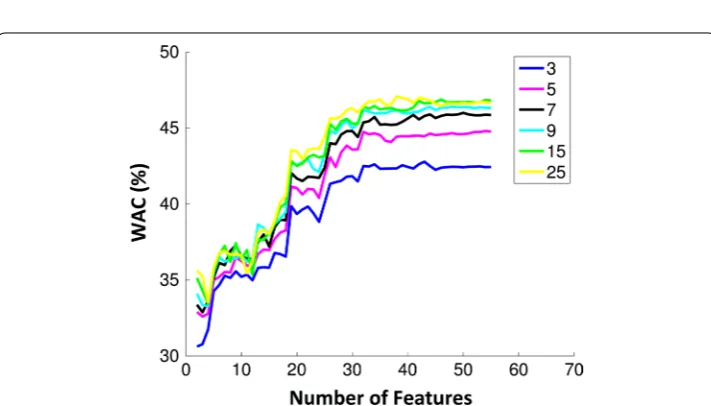
For the k-NN classifier different values of k [3, 5, 7, 9, 15, 25] were used to evaluate the performance. The behaviour of accuracy with the number of features is similar to the DA classifier. For the same number of features, the accuracy was similar independently of the
k value. However, WAC clearly depended on the number of neighbours, and the best k
that achieved higher weighted accuracy was 25, as depicted in Fig. 4. Considering a k-NN model with 30 features the mean values for WAC and AC were 46% and 70%, respectively. (12) WAC= 1
K K
Fig. 3 Evolution of WAC with the number of features used to build a model with LDA (L) and QDA (Q)
Fig. 4 Weighted accuracy evolution with the number of features using a k-NN classifier for different k-values [3, 5, 7, 9, 15, 25]
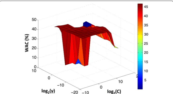
In both classifiers (DA or k-NN) the AC and WAC values stabilized after 30 features, independently of the classifier parameters. Since the computational cost increases with the number of dimensions used, the SVM models were build using only 40 features, which is a number that guaranties a good accuracy when DA and k-NN were applied. A grid search was performed for C=2−5, 2−3,. . ., 215 and γ =2−15, 2−13,. . ., 25 as pre-sented in Fig. 5. With this classifier, the best performance was obtained for C=2−1 and γ =2−1 , being 51% and 71% the mean WAC and AC, respectively.
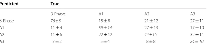
The confusion matrix represented in Table 3, shows that for SVM with C=2−1 and γ =2−1 , it can be seen that the B-phases were confused with the A1 and A2 subtypes in
with B-phase and 17% with A1. The A3 and A1 were the most distinct types, thus it was expectable that they were less confused.
PCA
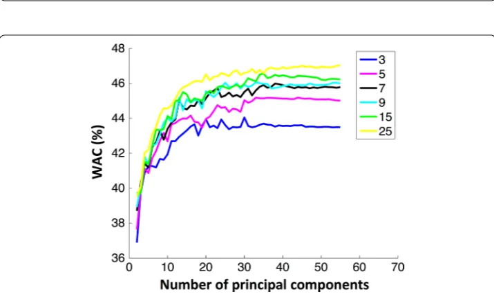
Using a DA classifier QDA achieved greater accuracy values than LDA, for all dimen-sions. More precisely, accuracy stabilized around 70% for more than 12 dimendimen-sions. Although the WAC significantly dropped for a classifier with more than 12 dimensions as can be observed in Fig. 6. A WAC of 49% was achieved using 12 components, that corresponded to an AC of 68%.
The results obtained with a k-NN classifier using PCA components was quite similar with the ones obtained with feature selection by mRMR, as presented in Fig. 7. Besides this similarity the performance using PCA started to stabilize for more than 30 compo-nents as when using mRMR. The WAC registered for 40 principal compocompo-nents and for k = 25 was 47%, corresponding to an AC of 61%.
Using features selected by mRMR both DA and k-NN started to stabilize for more than 30 dimensions. Although, when PCA was used for a DA classifier WAC achieved a maximum for 12 features and afterwards started to decrease. In k-NN the Table 3 Mean of confusion matrix for an SVM classifier using the 40 features ranked by mRMR, for the parameters of C = 2−1 and γ = 2−1
Italic font indicates the matrix main diagonal that represent the correctly predicted instances
Predicted True
B-Phase A1 A2 A3
B-Phase 76 ± 5 15 ± 8 21 ± 12 27 ± 11
A1 11 ± 4 59 ± 14 27 ± 13 17 ± 10
A2 11 ± 6 22 ± 12 44 ± 15 32 ± 11
A3 7 ± 2 5 ± 4 8 ± 8 24 ± 10
performance increased until 30 principal components, and for more principal com-ponents the performance remained almost constant. Given the previous results of DA and k-NN it was chosen to use a SVM classifier with the first 30 more important principal components. The WAC results obtained after a grid search are presented in Fig. 8. The best SVM parameters were C=2−5 and γ =2−9 , resulting in WAC and AC of 47% and 56%, respectively.
The confusion matrix is shown in Table 4. With mRMR feature selection the results are more dispersive than when using PCA, i.e. when a class was misclassified using PCA it was mostly confused with one class rather than with two. An interest-ing observation for the combination of SVM and PCA was that the majority of A1, 32%, were mistaken with A2 and only 5% and 2% were misclassified as B-phase and A3-phase, respectively. Contrarily, in mRMR 22% of the real A1 were wrongly classi-fied as A2 and 15% confused with B-phases.
Fig. 6 Evolution of WAC with the number of PCA principal components used to build a model with LDA (L) and QDA (Q)
Binary classification of A‑phase vs B‑phase
For the two-class problem, where it was only necessary to detect the A-phases from the B-phases without concerning the A-phase subtype, all the classifiers applied to the previous problem are analyzed in the following.
mRMR
With DA, the higher value of WAC was 72% with a LDA classifier, and using the 43 best features. The registered SP, SE and AC were: 65%, 78% and 67%, respectively. Using k-NN with k=25 the better performance values were obtained for 55 features, being AC equal to 75% and WAC equal to 80%. In these conditions, sensitivity and specificity were 82% and 68%, respectively. Considering the SVM with 40 features, the highest WAC achieved was 78% for C=2−1 and γ =2−1 , assuming AC, SP and SE
the values 76%, 79% and 77%, respectively.
Table 4 Mean of confusion matrix for a SVM classifier using 30 principal components, for the parameters of C = 2−5 and γ = 2−9
Italic font indicates the matrix main diagonal that represent the correctly predicted instances
Predicted True
B-Phase A1 A2 A3
B-Phase 61 ± 3 5 ± 2 9 ± 4 26 ± 9
A1 17 ± 4 60 ± 17 35 ± 12 25 ± 8
A2 16 ± 4 32 ± 15 53 ± 10 38 ± 9
A3 6 ± 2 2 ± 3 3 ± 3 13 ± 5
PCA
Combining the principal components with DA classifier the higher WAC obtained was 76% for a QDA with 15 dimensions. In this case SE, SP and AC were 79%, 74% and 73%, respectively. Regarding k-NN, the highest WAC, 75%, was achieved for 54 components and for k=25 . SE, SP and AC were 86%, 65% and 68%, respectively. For SVM the best result was for 40 principal components and for c=2−5 and γ =2−11 .
The achieved WAC was 75%, being AC, SE and SP: 73%, 76% and 73%, respectively.
Summary
Table 5 presents an overview of the results obtained with the different classifiers, with fea-ture selection or reduction, and for the binary or multi-class classification problem. One can observe that feature selection by mRMR led to the attainment of the best results in both classification scenarios. For the multi-class problem, the best classifier was SVM, and for the binary case k-NN was the one that attained the better performance.
Discussion
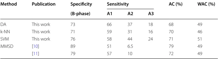
To the best of our knowledge, only two methods that discriminate between A-phases subtypes were found in literature, proposed by Barcaro et al. [11] and by Navona et al. [10]. In these methods, the subtypes A2 and A3 were joined and classified as one, A2/ A3. Aiming to improve comparison, the algorithms described in [10, 11] were imple-mented in this work and their results, as well as the results for the other methods, are compiled in Table 6. It can be seen that the sensitivities of A2/A3 were quite low, in the two versions proposed by Barcaro et al. (below 10%). Although, the AC of this method Table 5 Summary of the best results obtained for all the main methodological options considered
The best WAC results for each classification scenario (binary or multi-class) are in italic. #F. and #P. C. stand for number of features and number of principal components, respectively
Multi‑class problem Binary problem
mRMR PCA mRMR PCA
#F. AC (%) WAC (%) #P. C. AC (%) WAC (%) #F. AC (%) WAC (%) #P. C. AC (%) WAC (%)
DA 30 61 47 12 68 49 43 67 72 15 73 76
k-NN 30 70 46 40 61 47 55 75 80 54 68 75
SVM 40 71 51 30 56 47 40 76 78 40 73 75
Table 6 Comparison of the best classifier model proposed in this work with the ones presented in literature, that distinguish among A-phases subtypes
Method Publication Specificity Sensitivity AC (%) WAC (%)
(B‑phase) A1 A2 A3
DA This work 73 66 37 18 68 49
k-NN This work 71 59 31 16 70 46
SVM This work 76 58 44 24 71 51
MMSD [10] 89 51 6.5 79 49
was high. This value was due to class imbalance, i.e. due to a high predominance of the B-phases, which occupied 70% of the all data. Then, due to a high sensitivity of B-phases, AC will be high as well, even if the sensitivity of A-phases was low. WAC in turn was lower than AC, quantifying the low classification of the A2/A3 class. The KDD imple-mented for A-phases discrimination enabled the development of classification solutions to detect all the three A-phases subtypes, which is an innovation. All the A-phases sensi-tivities achieved were higher than the published methods.
Most of the A3 were arousals that are events with characteristics of awake sleep stage. Therefore, the classifiers were trained with B-phases similar to A3 phases, which led to a lot of A3 phases being wrongly classified as B-phase. This can be seen observing the confusion matrices represented in Tables 3, 4. The typical waveform associated with A1 are only the K-complex that counts with appropriate features for its detection, which explained the higher results for this subtype, compared to the A2 and A3.
Subtypes sensitivities can be improved by taking into account context information. Information from the macro-structure could be important to improve A3 discrimina-tion, given that it is confused with the awake state. Other aspect that is important to take into account is the subject condition. For example, NFLE patients, to which belongs the population considered in this work, are characterized by a significant enhancement of all A-phases subtypes when compared with controls [58]. In addition, A-phases offers favorable conditions for the occurrence of nocturnal motor seizures [6], and for the gen-eration of paroxysmal EEG features that can be used as bio-markers.
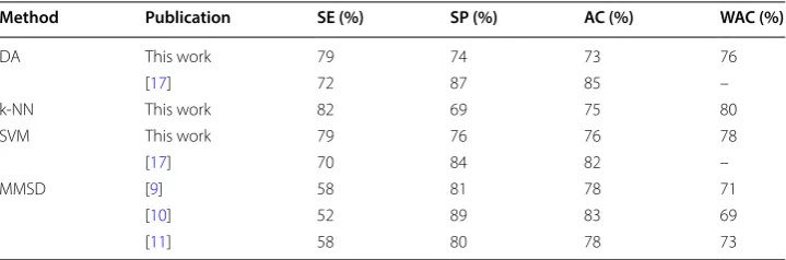
The majority of the algorithms presented in literature were developed for A-phase vs B-phase detection, as it can be seen in the literature review. The performance of the pro-posed algorithms with those in the literature are compared in Table 7.
In general, the accuracy reported in literature is higher than the ones reported in this work for the various methods. This is due to the fact that they reported the stand-ard accuracy without accounting for class imbalance. Therefore, again, they gave more importance to the B-phases that were more numerous than the A-phases. The consid-eration of WAC enabled a more appropriate estimation of the algorithms performance. In fact, if WAC was considered instead of AC, the algorithms presented in [9–11], pre-sented much lower performance values, as can be observed in Table 7.
Table 7 Comparison of the best classifier model proposed in this work with the ones present in literature to detect A-phases
Method Publication SE (%) SP (%) AC (%) WAC (%)
DA This work 79 74 73 76
[17] 72 87 85 –
k-NN This work 82 69 75 80
SVM This work 79 76 76 78
[17] 70 84 82 –
MMSD [9] 58 81 78 71
[10] 52 89 83 69
Conclusion
We propose a multi-step KDD to determine appropriate processing options for auto-matic CAP scoring. We extracted several features, approached two different feature selection/reduction methods, and different classification methods. It was concluded that using the features ranked by mRMR without any transformations leads to better results. It was shown that the SVM was the best classification method for the full discrimination of all CAP components, while k-NN performed better when one just wants to discrimi-nate A-phases from B-phases.
The proposed KDD is for the first time applied to CAP scoring. In particular, the fully discrimination of the three different A-phases subtypes is a new perspective, since past works tried multi-class approaches but based on grouping of different sub-types. We also considered the weighted accuracy, in addition to simple accuracy, resulting in a more trustworthy performance assessment. Globally, better subtype sensitivities than other published approaches were achieved.
Future steps to improve classification will encompass the consideration of context information related with CAP classification, as for example sleep stage and subject med-ical condition. Other future step is the analysis of the benefits of micro-structure staging as a disease biomarker, as for example as a precursor of epileptic seizures.
Authors’ contributions
FM implemented all the algorithms and performed the main analysis. FS and CS contributed with the clinical knowledge, including results validation. AD and CT supervised FM work and implemented major manuscript changes. All authors read and approved the final manuscript.
Author details
1 CISUC-Centro de Informática e Sistemas da Universidade de Coimbra, Departamento de Engenharia Informática, Faculdade de Ciências e Tecnologia, Universidade de Coimbra, 3030-290 Coimbra, Portugal. 2 Centro Integrado de Epi-lepsia, Centro Hospitalar e Universitário de Coimbra, Coimbra, Portugal. 3 Centro de Medicina do Sono do Hospital Geral Coimbra, Coimbra, Portugal.
Acknowledgements
Not applicable.
Competing interests
The authors declare that they have no competing interests.
Availability of data and materials
All of the datasets used in this article are freely available at https ://physi onet.org/pn6/capsl pdb/.
Consent for publication
Not applicable.
Ethics approval and consent to participate
We used a publicly available database; thus, this section is not applicable.
Funding
The authors would like to thank the financial support of Liga Portuguesa Contra a Epilepsia that awarded the scientific grant “EPICAP-Long-term evaluation of the cyclic alternating pattern (CAP) as a precursor of epileptic seizures”.
Publisher’s Note
Springer Nature remains neutral with regard to jurisdictional claims in published maps and institutional affiliations.
Received: 8 October 2018 Accepted: 11 December 2018
References
1. Parrino L, Ferri R, Bruni O, Terzano MG. Cyclic alternating pattern (CAP): the marker of sleep instability. Sleep Med Rev. 2012;16:27–45.
3. Terzano MG, Mancia D, Salati MR, Costani G, Decembrino A, Parrino L. The cyclic alternating pattern as a physiologic component of normal NREM sleep. Sleep. 1985;8(2):137–45.
4. Thomas RJ. Arousals in sleep-disordered breathing: patterns and implications. Sleep. 2003;26(8):1042–7. 5. Parrino L, Halasz P, Tassinari CA, Terzano MG. CAP, epilepsy and motor events during sleep: the unifying role of
arousal. Sleep Med Rev. 2006;10:267–85.
6. Parrino L, Smerieri A, Spaggiari MC, Terzano MG. Cyclic alternating pattern (CAP) and epilepsy during sleep: how a physiological rhythm modulates a pathological event. Clin Neurophysiol. 2000;111(SUPPL. 2):S39–46.
7. Terzano MG, Parrino L, Smerieri A, Chervin R, Chokroverty S, Guilleminault C, et al. Erratum: “Atlas, rules, and record-ing techniques for the scorrecord-ing of cyclic alternatrecord-ing pattern (CAP) in human sleep” (Sleep Med (2001) vol. 2 (6) (537–553)). Sleep Med. 2002;3(2):185.
8. Tatum WO. Ellen R. grass lecture: extraordinary EEG. Neurodiagn J. 2014;54(1):3–21.
9. Barcaro U, Navona C, Belloli S, Bonanni E, Gneri C, Murri L. A simple method for the quantitative description of sleep microstructure. Electroencephalogr Clin Neurophysiol. 1998;106(5):429–32.
10. Navona C, Barcaro U, Bonanni E, Di Martino F, Maestri M, Murri L. An automatic method for the recognition and clas-sification of the A-phases of the cyclic alternating pattern. Clin Neurophysiol. 2002;113(11):1826–31.
11. Barcaro U, Bonanni E, Maestri M, Murri L, Parrino L, Terzano MG. A general automatic method for the analysis of NREM sleep microstructure. Sleep Med. 2004;5(6):567–76.
12. Rosa AC, Parrino L, Terzano MG. Automatic detection of cyclic alternating pattern (CAP) sequences in sleep: prelimi-nary results. Clin Neurophysiol. 1999;110(4):585–92.
13. Largo R, Munteanu C, Rosa A. CAP event detection by wavelets and GA tuning. In: Intelligent signal processing, 2005 IEEE international workshop on, vol. 2, no. 1. 2005. pp. 44–8.
14. Stam CJ, Van Dijk BW. Synchronization likelihood: an unbiased measure of generalized synchronization in multivari-ate data sets. Phys D Nonlinear Phenom. 2002;163(3–4):236–51.
15. Ferri R, Rundo F, Bruni O, Terzano MG, Stam CJ. Dynamics of the EEG slow-wave synchronization during sleep. Clin Neurophysiol. 2005;116(12):2783–95.
16. Ferri R, Rundo F, Bruni O, Terzano MG, Stam CJ. Regional scalp EEG slow-wave synchronization during sleep cyclic alternating pattern A1 subtypes. Neurosci Lett. 2006;404(3):352–7.
17. Mariani S, Manfredini E, Rosso V, Grassi A, Mendez MO, Alba A, et al. Efficient automatic classifiers for the detection of A phases of the cyclic alternating pattern in sleep. Med Biol Eng Comput. 2012;50(4):359–72.
18. Goldberger AL, Amaral LAN, Glass L, Hausdorff JM, Ivanov PC, Mark RG, et al. PhysioBank, PhysioToolkit, and Physio-Net. Circulation. 2000;101(23):E215–20.
19. Ferri R, Bruni O, Miano S, Smerieri A, Spruyt K, Terzano MG. Inter-rater reliability of sleep cyclic alternating pattern (CAP) scoring and validation of a new computer-assisted CAP scoring method. Clin Neurophysiol. 2005;116(3):696–707.
20. Rechtschaffen A, Kales A. A manual of standardized terminology, techniques and scoring system for sleep stages of human subjects. Washington, DC: Public Heal Serv US Gov Print Off; 1968.
21. Iber C, Ancoli-Israel S, Chesson AL, Quan S. The AASM manual for the scoring of sleep and associated events: rules, terminology and technical specifications. Westchester, IL: American Academy of Sleep Medicine; 2007. p. 59. 22. Butterworth S. On the theory of filter amplifiers. Wirel Eng. 1930;7:536–41.
23. Kaleem M, Guergachi A, Krishnan S. Application of a variation of empirical mode decomposition and teager energy operator to EEG signals for mental task classification. In: Proceedings of the annual international conference of the IEEE engineering in medicine and biology society, EMBS. 2013. p. 965–8.
24. Kvedalen E. Signal processing using the Teager energy operator and other nonlinear operators. Signal Process. 2010;9120(May):121.
25. Bahoura M, Rouat J. Wavelet speech enhancement based on time-scale adaptation. Speech Commun. 2006;48(12):1620–37.
26. Jabloun F, Çetin AE, Erzin E. Teager energy based feature parameters for speech recognition in car noise. IEEE Signal Process Lett. 1999;6(10):259–61.
27. Lauer RT, Prosser LA. Use of the Teager–Kaiser energy operator for muscle activity detection in children. Ann Biomed Eng. 2009;37(8):1584–93.
28. Duman F, Erdamar A, Erogul O, Telatar Z, Yetkin S. Efficient sleep spindle detection algorithm with decision tree. Expert Syst Appl. 2009;36(6):9980–5.
29. Erdamar A, Duman F, Yetkin S. A wavelet and teager energy operator based method for automatic detection of K-Complex in sleep EEG. Expert Syst Appl. 2012;39(1):1284–90.
30. Carrozzi M, Accardo A, Bouquet F. Analysis of sleep-stage characteristics in full-term newborns by means of spectral and fractal parameters. Sleep. 2004;27(7):1384–93.
31. Cai H. Fast frequency measurement algorithm based on zero crossing method. In: ICCET 2010—2010 international conference on computer engineering and technology, proceedings. 2010.
32. Djurić MB, Djurišić ŽR. Frequency measurement of distorted signals using Fourier and zero crossing techniques. Electr Power Syst Res. 2008;78(8):1407–15.
33. Aye YY. Speech recognition using Zero-crossing features. In: Proceedings—2009 international conference on elec-tronic computer technology, ICECT 2009. 2009. p. 689–92.
34. Drinnan MJ, Murray A, White JE, Smithson AJ, Griffiths CJ, Gibson GJ. Automated recognition of EEG changes accom-panying arousal in respiratory sleep disorders. Sleep. 1996;19(4):296–303.
35. Lempel A, Ziv J. On the complexity of finite sequences. IEEE Trans Inf Theory. 1976;22:75–81.
36. Abásolo D, Simons S, Morgado da Silva R, Tononi G, Vyazovskiy VV. Lempel-Ziv complexity of cortical activity during sleep and waking in rats. J Neurophysiol. 2015;113(7):2742–52.
37. Casali AG, Gosseries O, Rosanova M, Boly M, Sarasso S, Casali KR, et al. A theoretically based index of consciousness independent of sensory processing and behavior. Sci Transl Med. 2013;5(198):198ra105.
• fast, convenient online submission
•
thorough peer review by experienced researchers in your field
• rapid publication on acceptance
• support for research data, including large and complex data types
•
gold Open Access which fosters wider collaboration and increased citations maximum visibility for your research: over 100M website views per year
•
At BMC, research is always in progress.
Learn more biomedcentral.com/submissions
Ready to submit your research? Choose BMC and benefit from:
39. Bracewell RN. The Fourier transform and its applications. New York: McGraw-Hill; 1986. p. 1–4.
40. Allen J. Short term spectral analysis, synthesis, and modification by discrete Fourier transform. IEEE Trans Acoust. 1977;25(3):235–8.
41. Ebrahimi F, Setarehdan SK, Ayala-Moyeda J, Nazeran H. Automatic sleep staging using empirical mode decomposi-tion, discrete wavelet transform, time-domain, and nonlinear dynamics features of heart rate variability signals. Comput Methods Programs Biomed. 2013;112(1):47–57.
42. Rutkowski TM, Mandic DP, Cichocki A, Przybyszewski AW. EMD approach to multichannel EEG Data—The amplitude and phase synchrony analysis technique. Lecture notes in computer science (including subseries Lecture notes in artificial intelligence and Lecture notes in bioinformatics). 2008. p. 122–9.
43. Kannathal N, Choo ML, Acharya UR, Sadasivan PK. Entropies for detection of epilepsy in EEG. Comput Methods Programs Biomed. 2005;80(3):187–94.
44. Chouvarda I, Mendez MO, Rosso V, Bianchi AM, Parrino L, Grassi A, et al. Predicting EEG complexity from sleep macro and microstructure. Physiol Meas. 2011;32(8):1083–101.
45. Chouvarda I, Mendez MO, Alba A, Bianchi AM, Grassi A, Arce-Santana E, et al. Nonlinear analysis of the change points between A and B phases during the Cyclic Alternating Pattern under normal sleep. In: Proceedings of the annual international conference of the IEEE engineering in medicine and biology society, EMBS. 2012. p. 1049–52. 46. Chouvarda I, Mendez MO, Rosso V, Bianchi AM, Parrino L, Grassi A, et al. CAP sleep in insomnia: new
methodologi-cal aspects for sleep microstructure analysis. In: Proceedings of the annual international conference of the IEEE engineering in medicine and biology society, EMBS. 2011. p. 1495–8.
47. Koley B, Dey D. An ensemble system for automatic sleep stage classification using single channel EEG signal. Com-put Biol Med. 2012;42(12):1186–95.
48. Rodríguez-Sotelo JL, Osorio-Forero A, Jiménez-Rodríguez A, Cuesta-Frau D, Cirugeda-Roldán E, Peluffo D. Automatic sleep stages classification using EEG entropy features and unsupervised pattern analysis techniques. Entropy. 2014;16(12):6573–89.
49. Higuchi T. Approach to an irregular time series on the basis of the fractal theory. Phys D Nonlinear Phenom. 1988;31(2):277–83.
50. Savitzky A, Golay MJE. Smoothing and differentiation of data by simplified least squares procedures. Anal Chem. 1964;36(8):1627–39.
51. Peng H, Long F, Ding C. Feature selection based on mutual information: criteria of max-dependency, max-relevance, and min-redundancy. IEEE Trans Pattern Anal Mach Intell. 2005;27(8):1226–38.
52. Shlens J. A tutorial on principal component analysis. arXiv Prepr arXiv14041100. 2014;1–13. .
53. Izenman AJ. Linear discriminant analysis. In: Modern multivariate statistical techniques. 2013. p. 237–80.
54. Altman NS. An introduction to Kernel and nearest-neighbor nonparametric regression. Am Stat. 1992;46(3):175–85. 55. Vapnik V, Chervonenkis A. Ordered risk minimization. Autom Remote Control. 1974;34:1226–35.
56. Duan K-B, Keerthi SS. Which is the best multiclass SVM method? An empirical study. Mult Classif Syst. 2005;3541:278–85.
57. Picard RR, Cook RD. Cross-validation of regression models. J Am Stat Assoc. 1984;79(387):575–83.