doi:10.5194/gmd-9-3907-2016
© Author(s) 2016. CC Attribution 3.0 License.
An approach to computing discrete adjoints for MPI-parallelized
models applied to Ice Sheet System Model 4.11
Eric Larour1, Jean Utke2, Anton Bovin3, Mathieu Morlighem4, and Gilberto Perez5
1Jet Propulsion Laboratory, California Institute of technology, 4800 Oak Grove Drive MS 300-323,
Pasadena, CA 91109-8099, USA
2Allstate Insurance Company, 2775 Sanders Rd., Northbrook, IL 60062, USA
3Department of Physics, The University of Chicago, 5720 South Ellis Avenue, Chicago, IL 60637, USA
4University of California, Irvine, Department of Earth System Science, Croul Hall, Irvine, CA 92697-3100, USA 5University of California, Irvine, School of Information and Computer Sciences, Irvine, CA 92697-3100, USA
Correspondence to:Eric Larour ([email protected])
Received: 26 April 2016 – Published in Geosci. Model Dev. Discuss.: 9 May 2016 Revised: 15 September 2016 – Accepted: 6 October 2016 – Published: 1 November 2016
Abstract.Within the framework of sea-level rise projections, there is a strong need for hindcast validation of the evolu-tion of polar ice sheets in a way that tightly matches obser-vational records (from radar, gravity, and altimetry observa-tions mainly). However, the computational requirements for making hindcast reconstructions possible are severe and rely mainly on the evaluation of the adjoint state of transient ice-flow models. Here, we look at the computation of adjoints in the context of the NASA/JPL/UCI Ice Sheet System Model (ISSM), written in C++ and designed for parallel execution with MPI. We present the adaptations required in the way the software is designed and written, but also generic adaptations in the tools facilitating the adjoint computations. We concen-trate on the use of operator overloading coupled with the Ad-joinableMPI library to achieve the adjoint computation of the ISSM. We present a comprehensive approach to (1) carry out type changing through the ISSM, hence facilitating operator overloading, (2) bind to external solvers such as MUMPS and GSL-LU, and (3) handle MPI-based parallelism to scale the capability. We demonstrate the success of the approach by computing sensitivities of hindcast metrics such as the misfit to observed records of surface altimetry on the northeastern Greenland Ice Stream, or the misfit to observed records of surface velocities on Upernavik Glacier, central West Green-land. We also provide metrics for the scalability of the ap-proach, and the expected performance. This approach has the potential to enable a new generation of hindcast-validated projections that make full use of the wealth of datasets
cur-rently being collected, or already collected, in Greenland and Antarctica.
1 Introduction
and bedrock elevation (Morlighem et al., 2014), among oth-ers. However, these approaches aim at improving our knowl-edge of poorly constrained input parameters and boundary conditions as long as the ice-flow regime is captured in a steady-state configuration. These inversions rely on analyti-cally derived adjoint states of forward stress balance or mass-transport models, but do not extend to transient regimes of ice flow.
Applications to transient models and long temporal time series such as the ICESat/CryoSat continuous altimetry record from 2003 to the present day have been much more rare, and, to our knowledge, are limited to a few studies such as Heimbach and Bugnion (2009), Goldberg and Sergienko (2011), Goldberg and Heimbach (2013), Larour et al. (2014), and Goldberg et al. (2015), among others. The main issue here precluding widespread application of transient data as-similation lies in the difficulty in deriving temporal adjoints of transient models. In many cases, the sheer number of phys-ical processes being represented makes the manual derivation of the adjoint state of a forward model extremely cumber-some and difficult to maintain. This state of affairs can be mitigated by adopting different approaches, such as (1) en-semble runs, as in Applegate et al. (2012), where model runs compatible with observations are selected; (2) methods simi-lar to the flux-correction methods implemented in Aschwan-den et al. (2013); Price et al. (2011), where boundary condi-tions are corrected in order to match time series of observa-tions (tuning approach); (3) quasi-static approaches, where snapshot inversions are carried out in time, as in Habermann et al. (2012, 2013); and (4) sampling methods, which have the main drawback of being computationally very expensive (each sample at the cost of one forward run). Though this is not an exhaustive list of all available methods, the main advantage of adjoint-driven inversions is that it relies on the exact sensitivity of a forward model to its inputs, hence en-suring a physically meaningful inversion.
Understanding sensitivities of a forward ice-flow model, which is needed to physically constrain a temporal inver-sion, requires computation of derivatives of model outputs to model inputs. If such derivatives are approximated by finite-difference schemes, they are subject to the tradeoff be-tween approximation and truncation errors for the pertur-bation, which is aggravated for higher-order derivatives. If the derivatives are computed using algorithmic differentia-tion (AD; Griewank and Walther, 2008), also known as au-tomatic differentiation, then one can attain derivatives at a floating-point precision equivalent to that of the underlying program implementation of the numerical model, provided it is amenable to the application of an AD tool. In particular, this approach does not depend on the type of physics relied upon, and it is transparent to the model equations, provided each step of the overall software is differentiable. Indeed, the
AD method assumes a numerical modelMthat is a function f :Rn → Rm
x 7−→ y=f(x) (1)
implemented as a computer program. The execution of the program implies the execution of a sequence of arithmetic operators such as+,−, and∗and intrinsics sin, ex, and so
forth to which the chain rule can be applied. For each such elemental operationr=φ (a, b, . . .)with resultr and argu-mentsa, b, . . .1we can write the total derivative as
˙
r=∂φ
∂aa˙+ ∂φ ∂b
˙
b+. . .. (2)
For example, ifφis the multiplication operator∗, i.e.,r=
ab, then one will get the product ruler˙=ba˙+ab. Applying˙ the above rule to each elemental operation in the sequence gives a method to compute
˙
y=Jx˙ with the Jacobian,
J=
∂f i ∂xj
, i=1. . .m, j=1. . .n,
without explicitly forming the Jacobian. This method applies the chain rule in the computation order of the values in the program and is known as forward-mode AD. The opposite order of applying the chain rule to the elemental operations, known as reverse or adjoint-mode AD, yields projections x=JTy.
This is achieved using the partial derivatives of the for-ward operationφas weights in redistributing the adjoints of the resultr to the adjoints of the respective argumentsa,b following the rule
a=a+∂φ
∂ar; b=b+ ∂φ
∂br; . . .r; =0. (3) Herevdenotes the adjoint corresponding to variablev. The final zeroing of the result adjointrcorresponds to the notion thatrhad been assigned a new value overriding any previous valuermight have had. Correspondingly the adjoint ofrhas been completely distributed, and to allow the increment for-mulation for the adjoint of any prior value ofr, it has to be (re)set to 0.
For the multiplication example one therefore gets a=
a+br; b=b+ar; r=0. In particular, for applications in
whichmn, the reverse mode is advantageous because its computational cost depends onmreverse sweeps instead ofn forward sweeps. Typical problems in cryosphere science in-volve computations of diagnostics that are scalar-valued cost functions (m=1), such as for example the spatio-temporally
averaged misfit between modeled surface elevation and ob-served surface topography (Larour et al., 2014). For these
cases, one can compute the gradient∇f =JTy withy=1
as a single projection (where f is the function defined in Eq. 1). Thus, for high-resolution models implying very large n, the reverse mode is an enabling and potentially very ef-ficient technique. This significant capability in AD is what makes its application to data assimilation so efficient. In-stead of evaluating a Jacobian using one forward sweep for each one of the model inputs, which would be significantly consuming as it scales in n, the reverse mode evaluates the gradient of one specific output of interest with respect to the model inputs in only one reverse sweep.
Using this approach, it is possible, without manual deriva-tion, to evaluate the derivative ∂f
∂xfrom Eq. (1). In cryosphere models,f could typically be a transient ice-flow model, with inputs x taken for example as the basal drag coefficient α at the ice–bed interface, and the outputy as the cost func-tion measuring the spatio-temporally averaged difference be-tween for example surface elevation and an altimetry record. In this case,m=1, andnis the number of degrees of free-dom of the basal drag input. Obtaining the sensitivity func-tion ∂f
∂x is critical both in terms of enabling data assimila-tion using inversion methods and in terms of understand-ing the sensitivity of a model to its model inputs, as well as the impact of processes represented in the model itself. Ap-proaches other than AD can be relied upon to compute such a sensitivity, such as solving for the adjoint equation directly (Morlighem et al., 2010; Larour et al., 2012; Cornford et al., 2013), but usually, a mix of forward AD or reverse AD is implemented for formulations where the manual derivation is difficult (Pawlowski et al., 2012; Goldberg and Heimbach, 2013). In Pawlowski et al. (2012) for example, AD relies on template-based generic programming to compute sensitivi-ties, while in Goldberg and Heimbach (2013), AD is based on source-to-source transformation. Our approach will in-stead be based on so-called operator overloading, which is uniquely suited to a framework written in C++.
Applying AD to large-scale frameworks such as the Ice Sheet System Model (ISSM) (Larour et al., 2012), MITgm (Heimbach, 2008), SICOPOLIS (Heimbach and Bugnion, 2009), or DassFlow (Monnier, 2010, among others) is a dif-ficult proposition but one that enables significant improve-ments in the way models can be initialized (Heimbach and Bugnion, 2009), hindcast validated (Larour et al., 2012), and calibrated (Goldberg et al., 2015) towards better projections. Traditional approaches relying on source-to-source transfor-mation have been developed, but for frameworks such as the ISSM, which are C++ oriented, and highly parallelized, this type of approach breaks down. Our goal here is to demon-strate how the so-called operator-overloading AD approach can be implemented and validated for a framework such as the ISSM, and what developments were necessary to make this capability operational. Our approach is discussed in Sect. 2 of this paper, with Sect. 3 describing the method vali-dation as well as applications with the ISSM. We discuss and conclude in the last section the applicability of such an
ap-proach to other frameworks, and the opportunities these new developments afford for cryosphere science and data assimi-lation of remote sensing data in particular.
2 Methodology and validation
2.1 Source-to-source vs. overloaded operators
Distinctions between the AD implementation approaches re-late to the way the derivative data inv˙orv, respectively, are
associated with the original program variablev (data aug-mentation) and how the logic for coefficient propagation is added to the original program (logic augmentation). The ba-sic options for the former are association by address and as-sociation by name. Asas-sociation by address packs the origi-nal and the derivative data into a new type called the active type, and all differentiated program variables have their type changed to that new active type. For the logic augmentation one uses source code transformation or operator overload-ing. Because of the complexity of the C++ syntax and se-mantics, there currently still is no comprehensive AD tool for source code transformation of C++ models, and thus op-erator overloading remains the method of choice, implying association by address for the data augmentation. In prac-tice, the overloaded operators and intrinsics for the forward mode typically execute Eq. (2) directly for the forward mode and for the reverse mode record the sequence of operations into a traceT (f (x)), which then is read backward by an in-terpreterR(T )that executes the statements Eq. (3) for the reverse mode. The invocation of R(T ) is part of the user-written logic that then uses the derivatives. The model thus enhanced by an adjoint capability computing bothf and∇f is denoted byM.
2.2 Type change to enable overloaded operators Changing to the aforementioned active type is a significant effort to be undertaken in the model code. Among the choices to effect this type change, one should select one that is trans-parent to the model development process, is maintainable, and minimizes the manual effort.
fac-tor in the computational efficiency of the adjoint. Thus, one must categorize program variables intoAandPwith the aim of minimizing the set A of active (i.e., type-changed) pro-gram variables. In the ISSM this is accomplished by chang-ingdoublevariables to a type named for brevity, e.g.,TA (in the ISSMIssmDouble) for variables inA, and to, e.g., TP(in the ISSMIssmPDouble) for variables inP, respec-tively. This categorization must be performed by an expert fa-miliar with the global data dependencies inMand the work that has been done forM. In addition, it can be incrementally done for code contributions supplied as doublevariables without breakingM. This is a key aspect of the overloaded AD approach that is amenable to easy maintenance and ex-pansion of a complex C++ framework such as the ISSM, and one of the key reasons why this approach was selected to compute M in the ISSM. In the end, alldoubletypes should eventually be replaced with eitherTAorTP. Follow-ing good practices in C++ bothTAandTParetypedefed in a central location switched only there via a preprocessing macro to use the active type supplied by the AD tool or hide the distinction altogether for running the plain M. This im-plies that one cannot explicitly overload methods or define data structures for distinctTA andTPwithout filtering the declaration and definition of theTAvariant by the preproces-sor as well. Such code duplication introduces an undue code maintenance burden.
Instead, the recommended approach is the use of C++ tem-plate classes and methods where TA andTP are the con-crete arguments for an abstract template type T. While the use of templates may imply a larger up-front effort if they were not present in the model code before, as was the case in the ISSM, the long-term benefits not only for M but also the plain M are obvious when one wants to experi-ment with computation at different precision levels. Aside from the ISSM, an established general example of this kind of templating is the use of SACADO within Trilinos (The Trilinos Project, 2014; Phipps et al., 2008). Of particular value in the ISSM was the migration of data containers for arrays and (sparse) matrices and that of existing wrappers to malloc andfree to templated wrappers of newand delete, calledxNewandxDeletein the ISSM. The lat-ter is necessary not only to properly instantiateTAvariables, but also permits specializations forTAinMas explained in the following.
Overall, the use of C++ template classes introduces an ad-ditional element of complexity to the code, but it also means that the same exact framework can be used to compute both the forward run and its gradient, using the exact same code base, without the need to manage different code for the com-putation ofM. This in turn means that the ISSM can be com-piled using ADOLC and shipped to the community in only one binary version that can accommodate both M andM, which is a critical feature in terms of extending AD features to the wider community without having to dive into the in-trinsic complexities of AD transformation itself.
Interpreting the trace byR(T )means that the space hold-ing the data for the variablesr, a, b∈V∗(the set of
instan-tiated program variables at runtime) occurring in each op-eration r=φ (a, b) must be represented by some mapping ω:V∗7−→
N+ to pseudo addresses. In ADOL-C these
ad-dresses are called locations and represent indices in a work array held byR(T ). The pseudo addresses must be managed through theTAconstructor and destructor in a fashion sim-ilar to the memory management of the actual program vari-ables themselves; i.e., pseudo addresses are assigned from and returned to a pool of available addresses. However, no distinction between heap and stack variables is made and generally data locality will not be preserved. On the other hand, for special operationsφAwith array arguments of size s, that is, calls to external solvers (see Sect. 2.3) or MPI rou-tines (see Sect. 2.4), it would be counterproductive to record inT the pseudo addresses of each of the s array elements rather than a consecutive range. The latter, however, requires that the pool be primed by some call(s)such thatω re-turns consecutive pseudo addresses when called by the con-structor for each element in the array. In ADOL-C this is done by callingensureContiguousLocations imme-diately before an active array is instantiated. Avoiding copy-ing of array values inMas an efficiency measure means that any given array has a good chance of being used inφA, and to avoid littering the code with preprocessor-guarded calls to(s), we decided in the ISSM to instead add a call to ensureContiguousLocations in the TA specializa-tion ofxNew:
#if defined(_HAVE_ADOL_C_) template <>
adouble* xNew(unsigned int s) { ensureContiguousLocations(s); adouble* aT_p=new adouble[s]; assert(aT_p);
return aT_p; }
#endif
Thus, the use ofφAmeans frequent calls to(s). The im-plementation of(s)searches the pool to find a sufficiently large consecutive range or otherwise grow the pool by at leastsaddresses. In the ISSM, this search became a signif-icant performance bottleneck. Minimizing the search effort and balancing it with pool growth has been newly imple-mented in ADOL-C and is controlled by setting parameters viasetStoreManagerControlfor the ratio of the ad-dresses inside and outside of the pool and the maximal pool size to trigger searches.
2.3 Binding to external solvers
to manually programming adjoints that are error-prone, and implies a significant effort in terms of code development and maintenance. However, because models reference libraries, for fixed mathematical mappings that may have easily pro-grammable high-level adjoints, one can and should exploit this insight as it can yield efficiency gains not obtainable by an AD tool remaining unaware that calls to some col-lection of subroutines represent a certain mathematical map-ping. A good example are linear solver libraries that may not even be written in the same programming language as the model in question. Considering the system As=b, the
solverScomputings=S(A, b)needs an adjoint counterpart solvingATt=s, incrementingb=b+tand, ifA∈A, also A=A−bsT. Clearly, the solve with the transposed can eas-ily be implemented reusing the solverS as int=S(AT, s). However, the answers to the following questions affect the efficiency and ought to be considered in the context of the given model (Giles, 2008).
Q1: IsA∈A, which therefore requires the rank-1 update to A?
Q2: Are the previous values ofs,r, andAoverwritten byS but used to compute partial derivatives for Eq. (3), and therefore must be saved and restored?
Q3: If S is a direct solver, should one save the factors or refactorize for the adjoint solve?
Q4: How does the external function interface used byR(T ) allow for efficient reuse of intermediate buffers? External functionsfethat had been supported by
ADOL-C had the signaturefe(lx, x, ly, y)with inputsx, outputsy for the original call,lx, ly for their respective array lengths, andfe(ly, y, lx, x)for the adjoint counterpart. In the case of a linear system withA∈A, the inputx is packed with both A andr, while y contains the solution s of the system on return. This, however, was insufficient for binding to solvers from the GNU Scientific Library (GSL; Galassi, 2009) and MUMPS (Amestoy et al., 2001) used by the ISSM. The fol-lowing extensions were implemented in ADOL-C to enable the ISSM adjoints, but are generic in nature and would need to be supported in some form by other tools.
E1: expanded thefeinterface byx, y tofe(ly, y, lx, x, x, y) to enable refactoring;
E2: added optional parameters to pass in the sparsity pattern ofAfor MUMPS as a generic integer arrayiof length lifor bothfeandfe;
E3: added controls for storing and restoring prior values of xandy;
E4: added tracking of the maximallx, lyin sequences offe calls.
Regarding Q1, we know that in the ISSM,A∈A, and re-garding Q2, the parameters passed tofehave no other uses
and, therefore, using the controls (E3), we avoid (re)storing their values. The direct solver from the GSL used here had no API control to back-solve with the factors for the transposed and we did not want to reverse engineer the permutation rep-resentation. Hence the refactoring was done as a matter of convenience for the sequential reference case requiring E1. The parallel and therefore practically more efficient MUMPS solver operates on sparse, distributedA, therefore requiring E2. MUMPS offers both the ability to store the factors to file and perform the back-solve for the transpose. However, the MUMPS portion of the runtime is comparatively small (see Sect. 3). Consequently the overhead for the file I/O when considering the factor data size after fill-in is not expected to yield much practical benefit in this context, answering Q3. Finally, for Q4, extension E4 is exploited because transient runs of the ISSM need to account for changes in the system size, and a preallocation with the maximal buffer sizes there-fore avoids some of the memory management overhead. 2.4 Handling parallelism with the AdjoinableMPI
library
As is the case with the ISSM, practically relevant science problems incur a computational complexity that necessi-tates execution on parallel hardware, often using MPI as the paradigm of choice. Sending data with MPI from a source buffers to a target buffer t can be interpreted as a simple assignmentt=s. This implies for the adjoint an increment
s=s+t; that is, the adjoint of a communication is a rever-sal of the data flow between buffers. Calculating the adjoint oft=s means sending back the value oft and computing s=s+t. The principles for adjoining two-sided MPI com-munication have been explored in Utke et al. (2009). The development of the AdjoinableMPI (AMPI) wrapper library AdjoinableMPI (2016) started in the fall of 2012. It is de-signed to provide an AD tool-independent implementation for adjoining MPI-parallelized C, C++, and Fortran models. The wrapper interfaces distinguish themselves from the orig-inal MPI by the prefixAMPIand have a few additional pa-rameters where needed to enable the adjoint functionality. AMPI also provides additional types and predefined sym-bols. Discussing the internal design of AMPI is outside the scope of this paper. However, the application to the ISSM is the first large-scale practical use of AMPI and in the follow-ing we will discuss the steps taken to use it in the ISSM code base.
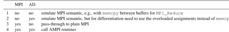
de-Table 1.Logic variants encapsulated in the ISSM MPI wrapper library.
MPI AD
1 no no emulate MPI semantic, e.g., withmemcpybetween buffers forMPI_Reduce
2 no yes emulate MPI semantic, but for differentiation need to use the overloaded assignments instead ofmemcpy 3 yes no pass-through to plain MPI
4 yes yes call AMPI routines
cided to introduce in the ISSM another wrapper layer (pre-fixed ISSM_MPI) of calls and definitions to encapsulate completely the four functionality variants listed in Table 1.
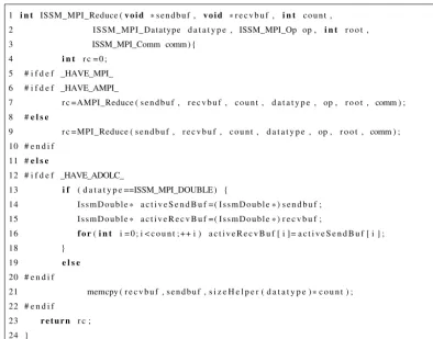
The approach is shown forMPI_Reducein Fig. 1. Variant 1 is implemented by line 21, variant 2 by lines 13– 18 and 21, variant 3 by line 9, and variant 4 by line 7. The example code reflects some of the simplifying assumptions being made based on the MPI usage patterns in the ISSM. Examples are the absence of MPI_IN_PLACE and user-defined MPI types as well as all active data being of double precision. This permits the simple distinction in line 12, but of course the logic covers all other non-differentiated MPI types that may occur. The following lines (14, 15) indicate the pairing between the C++ type definitionIssmDouble and the wrapper-definedISSM_MPI_DOUBLEto signify ac-tive data being communicated when AD is enabled. Mir-roring in MPI the approach described in Sect. 2.2 with two types TA and TP, the passive type TP (concrete IssmPDouble) has an MPI counterpart defined in the wrapper as ISSM_MPI_PDOUBLE. It too can be the value passed in via thedatatypeargument at line 1 and signals to AMPI passive floating-point communications. The defini-tions provided by theISSM_MPIwrapper corresponding to typesTAandTPare given in Table 2.
The matching between the actual type of the buffer and the corresponding MPI type must extend to the templating approach suggested for the type change in Sect. 2.2. The main reason is to avoid type errors, which become more common as the complexity of a code increases. Because the MPI standard keeps the definition ofMPI_Datatype opaque and MPI types can be created at runtime, the value of MPI_Datatypecannot be used as the value template parameter itself (as it may not be a compile time constant). Therefore, a template buffer typeTmust be paired with the corresponding MPI type value declared as a pointer parame-ter, as shown in Fig. 2. Assuming many AMPI calls infoo, this confines the code locations where type errors may be in-troduced to the template instantiations themselves.
Finally, a practical concern for using the parallelized ad-joint is the handling of sensitivities to quantities that are uniformly initialized across ranks, such as parameters. Fre-quently, as was the case within the ISSM, these quantities are initialized from files or otherwise per process in the parallel case the same way as in the sequential case. In the parallel case that implies a replication of the same quantity across
ranks. However, to obtain the correct sensitivities, the quan-tityqin question should be unique; in other words, that quan-tity must be uniquely initialized at one root rank and then broadcast to the other ranks. Otherwise, forrranks, at each rank one would then obtain only a partqi of the totalq and would have to “manually” sum upq=P
qi. With an initial broadcast ofq, however, the corresponding adjoint provided through AMPI by usingAMPI_Bcastis that exact sum re-duction, and R(T ) yields the correct adjoint at the broad-cast root. This notion similarly applies to any situation where a conceptually unique quantity of active type is implicitly replicated on some ranks.
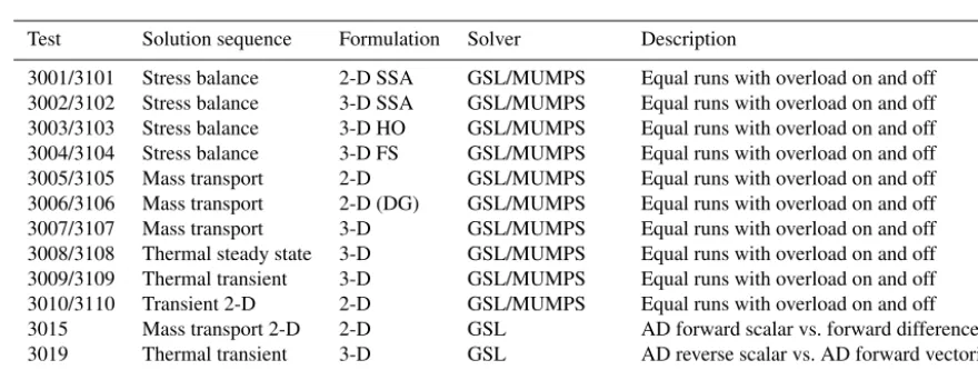
2.5 Validation
The ISSM is validated in AD mode by continuously run-ning a test suite within the Jenkins (Smart, 2011) integration and development framework (available here at http://issm.jpl. nasa.gov/developers/). A detailed description of the suite of benchmarks is given in Table 3. The aim is to (1) compare forward runs in the ISSM with their counterparts when over-loaded operators are switched on (the results should be iden-tical within double-precision tolerances); and to (2) compare forward and reverse runs carried out with the ISSM AD on and off, using the GSL and MUMPS solvers. Comparisons of gradients computed in AD mode with standard forward difference methods are also carried out to make sure the gra-dients computed (essentially in reverse scalar mode, which is the mode of predilection in the ISSM for data assimilation) in AD mode are accurate.
3 Application 3.1 Application
1 i n t ISSM_MPI_Reduce (void * sendbuf , void * r e c v b u f , i n t count , 2 ISSM_MPI_Datatype d a t a t y p e , ISSM_MPI_Op op , i n t r o o t ,
3 ISSM_MPI_Comm comm) {
4 i n t r c =0;
5 # i f d e f _HAVE_MPI_ 6 # i f d e f _HAVE_AMPI_
7 r c =AMPI_Reduce ( sendbuf , r e c v b u f , count , d a t a t y p e , op , r o o t , comm ) ; 8 #e l s e
9 r c =MPI_Reduce ( sendbuf , r e c v b u f , count , d a t a t y p e , op , r o o t , comm ) ; 10 # e n d i f
11 #e l s e
12 # i f d e f _HAVE_ADOLC_
13 i f ( d a t a t y p e ==ISSM_MPI_DOUBLE ) {
14 IssmDouble * activeSendBuf =( IssmDouble *) sendbuf ; 15 IssmDouble * activeRecvBuf =( IssmDouble *) r e c v b u f ;
16 f or(i n t i =0; i < c o u n t ;++ i ) a c t i v e R e c v B u f [ i ]= a c t i v e S e n d B u f [ i ] ;
18 }
19 e l s e
20 # e n d i f
21 memcpy ( r e c v b u f , sendbuf , s i z e H e l p e r ( d a t a t y p e ) * count ) ; 22 # e n d i f
23 return r c ; 24 }
Figure 1.Code for wrapping reduction.
/ / t h i s d e c l a r a t i o n comes from t h e wrapper :
extern ISSM_MPI_Datatype ourISSM_MPI_DOUBLEVal , ourISSM_MPI_DOUBLEVal ;
template <c l a s s T , ISSM_MPI_Datatype *mt_p> void foo ( T * t ){ ISSM_MPI_Reduce ( t , . . . , ,* mt_p , . . ) ;
}
void b a r ( IssmDouble *x , IssmPDouble *p ) { foo <IssmDouble ,&ourISSM_MPI_DOUBLEVal >( x ) ; foo <IssmPDouble ,&ourISSM_MPI_PDOUBLEVal >( p ) ; }
Figure 2.Code snippets for templating with corresponding MPI data types.
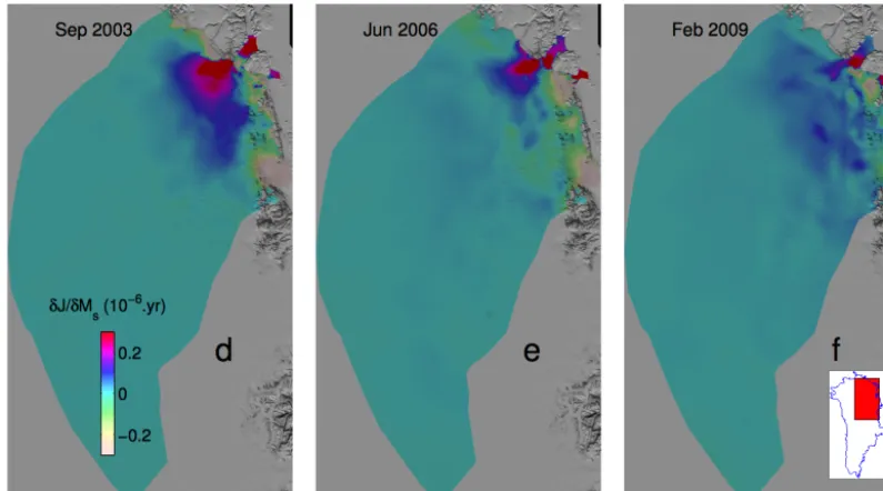
for three epochs, September 2003, June 2006, and Febru-ary 2009. The cost functionJAltimetry is the spatio-temporal average of the misfit between modeled surface elevations (from the mass-transport module of the transient solution in the ISSM) and the corresponding ICESat-1 altimetry record. This cost function was used within an inversion method to re-construct SMB over the entire ICESat-1 time record (Larour et al., 2014). This example would correspond to the case where functionf from Eq. (1) is a transient ice-flow model
(including mass transport and stress balance, not thermal, de-scribed in Larour et al., 2014), fully nonlinear in its treat-ment of the material rheology, and highly resolved both spa-tially (kilometer resolution at the coastline) and temporally (2-week time step). The final output (corresponding toy in Eq. 1) of the model is the altimetry cost functionJAltimetry
com-Table 2.Types per variant from Table 1.
ISSM_MPI_DOUBLE IssmDouble(=TA) ISSM_MPI_PDOUBLE IssmPDouble(=TP)
#defineto typedefto #defineto typedefto
1 2 double 3 double
2 2 adouble1 3 double
3 MPI_DOUBLE double MPI_DOUBLE double
4 AMPI_ADOUBLE2 adouble1 MPI_DOUBLE double
1Active type from ADOL-C.2Active MPI type from AMPI.
Table 3.ISSM AD validation suite integrated within Jenkins for continuous integration and delivery (Smart, 2011). Tests 3001 to 3010 and 3101 to 3110 test the repeatability of forward runs with and without ADOL-C compiled, but with no AD drivers specifically called. The forward runs involved are the standard stress balance, mass transport, and thermal solutions, with 2-D SSA (shelfy-stream approximation MacAyeal, 1989), 3-D SSA, 3-D HO (higher-order, Blatter, 1995; Pattyn, 1996), 3-D full-Stokes (Stokes, 1845), and DG (discontinuous-Galerkin) formulations. Test 3015 tests the AD GSL capability by comparing the AD forward scalar mode (where we compute the gradient of ice volume with respect to ice thickness at one vertex of the mesh) against a simple forward differences computation on the same gradient. Test 3019 validates the AD GSL capability in reverse scalar mode (where we compute ice volume gradient with respect to thickness at all vertices of the mesh) vs. the forward vectorial mode. Both gradients should be identical. Finally, test3119 validates the parallel capabilities (AD MUMPS) by comparing reverse scalar computations with GSL and MUMPS.
Test Solution sequence Formulation Solver Description
3001/3101 Stress balance 2-D SSA GSL/MUMPS Equal runs with overload on and off 3002/3102 Stress balance 3-D SSA GSL/MUMPS Equal runs with overload on and off
3003/3103 Stress balance 3-D HO GSL/MUMPS Equal runs with overload on and off
3004/3104 Stress balance 3-D FS GSL/MUMPS Equal runs with overload on and off
3005/3105 Mass transport 2-D GSL/MUMPS Equal runs with overload on and off
3006/3106 Mass transport 2-D (DG) GSL/MUMPS Equal runs with overload on and off
3007/3107 Mass transport 3-D GSL/MUMPS Equal runs with overload on and off
3008/3108 Thermal steady state 3-D GSL/MUMPS Equal runs with overload on and off
3009/3109 Thermal transient 3-D GSL/MUMPS Equal runs with overload on and off
3010/3110 Transient 2-D 2-D GSL/MUMPS Equal runs with overload on and off
3015 Mass transport 2-D 2-D GSL AD forward scalar vs. forward differences
3019 Thermal transient 3-D GSL AD reverse scalar vs. AD forward vectorial
3119 Thermal transient 3-D MUMPS vs. GSL AD reverse scalar (MUMPS vs. GSL) scalar
puted ∂JAltimetry
∂SMB at different time steps corresponding to the transient model input SMB.
A second type of observation garnering considerable inter-est is temporally resolved time series of radar observations (using speckle-tracking or InSAR to infer surface deforma-tion of the ice) to measure variadeforma-tions of surface velocity on a seasonal timescale (one observation every 2 months, as in Moon et al., 2015). Temporally inverting for such time series, trying to reconstruct for example basal friction, is a topic of interest due to its relevance in terms of understanding the dynamics of calving, basal slip, and shear softening, and as-sociated feedback mechanisms. In Fig. 4, we demonstrate the feasibility of such inversions by computing the gradient of a cost functionJVelocityrelated to the Moon et al. (2015) time series with respect to basal drag α at epochs 2008, 2010, and 2013. The cost function is the spatio-temporal average of the misfit between modeled surface velocity (from the stress balance module of the transient solution in the ISSM) and observed surface velocities. This example would correspond
to the case where functionf from Eq. (1) is the same tran-sient ice-flow model described previously, and the final out-put (corresponding toyin Eq. 1) of the model is the velocity cost functionJVelocityitself and the model input basal friction α(corresponding toxin Eq. 1). The sensitivity displayed in Fig. 4 is therefore the AD computed∂JVelocity
∂α at different time steps corresponding to the transient model inputα.
3.2 Benchmarking
Figure 3.Gradient of the surface altimetry cost function (spatio-temporal average of the misfit between the 6-year record of observed ICESat altimetry and modeled surface elevation) with respect to SMB (in years). The gradient is computed for every time step of a 2-week interval time series between 2003 and 2009. We only show three periods (September 2003, June 2006, and February 2009) in the entire interval. The location for the study is the northeastern Greenland Ice Stream, and the gradient is taken from an inversion study of the surface forcings necessary to best fit the ICESat altimetry record (Larour et al., 2014).
2008 2010 2013
Figure 4.Gradient of the surface velocity cost function (spatio-temporal average of the misfit between a 5-year time series of observed surface velocities and the modeled surface velocity) with respect to the basal drag coefficient (in yr1/2m−5/2). The gradient is computed for
every time step of a 2-week interval time series between 2008 and 2013. We only show three periods (2008, 2010, and 2013) in the entire interval. The location for the study is Upernavik Glacier, central West Greenland, and the gradient is taken from an inversion study of the basal forcings required to match observed RADAR time series of surface velocities and calving front positions.
to that the overhead incurred by calling the overloaded op-erators as well as the creation, storage, and interpretation of the traceT (as the means to compute∇f) on the other. Aside from the fact that the tuning of the ISSM adjoint is a work in progress, we want to highlight the overwhelming impact of the application-specific aspects on the runtime ratio. There-fore, we emphasize that exhibiting any particular overhead number as the ultimate result of scenario-specific tuning is of little use to the practitioner wanting to answer science ques-tions. Rather, using examples from the ISSM work, we want
to show what may prevent us from achieving a satisfactory overhead.
The earliest ISSM adjoint computations took place be-fore the MPI wrapper library was introduced and therebe-fore were done sequentially with the GSL solvers. To evalu-ate the performance, a representative test case was chosen from the ISSM regression test suite, test 101. This test mod-els the steady-state stress balance of a square ice shelf of size 50 km×50 km and thickness 1000 m (at the grounding
0 2 4 6 8 10 12 14
100 50 25 12.5
OO
Overloading overhead Trace overhead
0 0.2 0.4 0.6 0.8 1
100 50 25 12.5
libadolc libgsl I/O
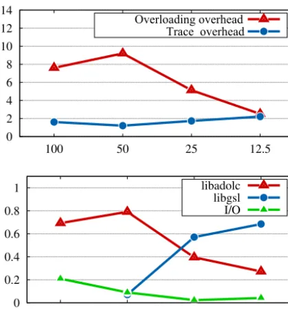
Figure 5.Test problem setup with the sequential GSL solver; plots over max mesh distance show overhead factors (upper frame) and approximate runtime portions of the model execution with adjoint computation (lower frame).
0 0.2 0.4 0.6 0.8 1
100 50 25 12.5 libadolc
libmumps
I/O
0.5 1 1.5 2
100 50 25 12.5
T
Trace overhead
Figure 6.Test problem setup with the parallel MUMPS solver; plots over max mesh distance show approximate runtime portions of the model execution with adjoint computation (upper frame) and over-head factors for the trace creation and interpretation (lower frame).
at the grounding line, free to flow at the ice front (on one side only), with nonlinear viscosity dependent on Glen’s law (Glen, 1955, 1958). The formulation relies on the shelfy-stream approximation (SSA, MacAyeal, 1989), and is inher-ently nonlinear, relying on a Picard iteration for convergence. For more details on this test, we refer the reader to Larour et al. (2012). For benchmarking, the problem size was in-directly set by specifying a measure for the maximal res-olution of the generated mesh, thus increasing the number
of mesh elements generated for a smaller-resolution param-eter. The parallel runs were carried out using eight CPUs. The overhead factors are shown separately for the overload-ing as such and the generation ofT andR(T )as wall-clock comparisons to the unmodified model compiled with default optimization (−O2) in Fig. 5 (upper frame). While this plot
indicates a small overhead factor of≈4.5 in particular for
the largest mesh case (distance 12.5 km), the reason for this becomes apparent in the plot in the lower frame. It shows that the majority of the runtime is consumed by the GSL solver (libgsl), completely overshadowing any of the over-head caused by the adjoint for the largest mesh. We want to emphasize that GSL was chosen not for its efficiency, but for the simplicity of the setup, which quickly enabled ad-joint computations. Introducing AMPI and thereby moving to a more appropriate solver (MUMPS) causes the adjoint overhead to become more prominent. The most consequen-tial change necessitated by the use of MPI is the forced con-tiguity of the pseudo addresses (see Sect. 2.2).
In combination with the much reduced impact of the solver, the overhead factor for equivalent test problems reached temporarily up to 145, which clearly was not ac-ceptable. Subsequent changes to the ADOL-C tool included improvements in the internal address management. Changes to the model included modifications of the sparse data for-mat, enabling the control of the I/O buffering for the traceT and the ADOL-C address manager via the ISSM configura-tion specific to the setup to be computed. The combinaconfigura-tion of these changes led to regaining of better performance and effective overall overheads between 10 and 30. Analyzing the details of the performance shows that the overhead fac-tor for the trace creation and interpretation does not change significantly (see Fig. 6, bottom) with the mesh size, in accor-dance with the theoretical result for the adjoint computation. The large majority of the total overhead, evidenced by the runtime portion for libadolc in Fig. 6 (top), still originates in the internal address management. While the overall over-head factors are sufficiently small for the practical use of the adjoints for science problems, further improvements in the addressing scheme are clearly warranted and the subject of ongoing work.
4 Conclusions
applica-ble or may prove more cumbersome. The flexibility of this approach allows in particular for quick turn-around in de-veloping adjoint models of new parameterizations that are not easily hand-derived. This is a major advantage in that it opens this approach to the wider community. This, given the large amount of remote sensing data currently being col-lected and under-utilized, could prove paramount if we are to hindcast validate projections of sea-level rise. Further work is of course required to bring in additional observations such as gravity sensors, or radar stratigraphy observations, which will involve development of new cost functions, and scal-ability in 3-D. Though this is complex in that it requires integrated resiliency and adjoint checkpointing schemes for long-running transient modeling scenarios, our approach has proven flexible, and should lead to a brand new set of data assimilation capabilities that have already been available to other Earth science communities for a long time. Indeed, by allowing temporal data assimilation for a large number of sensors and models, such as demonstrated here with the use of altimetry and radar sensors for mass transport and stress balance models, respectively, the ISSM paves the way for wider integration between the modeling and observational cryosphere communities.
5 Code availability
The ISSM code and its AD components are available at http: //issm.jpl.nasa.gov. The instructions for the compilation of the ISSM in AD mode, along with test cases, are presented in the Supplement attached to this paper.
The Supplement related to this article is available online at doi:10.5194/gmd-9-3907-2016-supplement.
Acknowledgements. DE-AC02-06CH11357. Eric Larour and Jean Utke were supported by the Jet Propulsion Laboratory, California Institute of Technology, under a contract with the NASA Cryospheric Sciences and Modeling and Analysis Programs. Gilberto Perez was supported by a subcontract from the Jet Propulsion Laboratory to the University of California at Irvine and Mathieu Morlighem was supported under a contract with the NASA IceBridge research program.
Edited by: D. Goldberg
Reviewed by: L. Hascoet and one anonymous referee
References
AdjoinableMPI: AdjoinableMPI wiki, https://trac.mcs.anl.gov/ projects/AdjoinableMPI/wiki, last access: 19 October 2016. ADOL-C: ADOL-C, http://www.coin-or.org/projects/ADOL-C.
xml (last access: 19 October 2016), 2007.
Amestoy, P. R., Duff, I. S., Koster, J., and L’Excellent, J.-Y.: A Fully Asynchronous Multifrontal Solver Using Distributed Dynamic Scheduling, SIAM J. Matrix Anal. Appl., 23, 15–41, 2001. Applegate, P. J., Kirchner, N., Stone, E. J., Keller, K., and Greve, R.:
An assessment of key model parametric uncertainties in projec-tions of Greenland Ice Sheet behavior, The Cryosphere, 6, 589– 606, doi:10.5194/tc-6-589-2012, 2012.
Arthern, R. J. and Gudmundsson, G. H.: Initialization of ice-sheet forecasts viewed as an inverse Robin problem, J. Glaciol., 56, 527–533, 2010.
Aschwanden, A., Aðalgeirsdóttir, G., and Khroulev, C.: Hindcast-ing to measure ice sheet model sensitivity to initial states, The Cryosphere, 7, 1083–1093, doi:10.5194/tc-7-1083-2013, 2013. Bindschadler, R., Nowicki, S., Abe-Ouchi, A., Aschwanden, A.,
Choi, H., Fastook, J., Granzow, G., Greve, R., Gutowski, G., Herzfeld, U., Jackson, C., Johnson, J., Khroulev, C., Levermann, A., Lipscomb, W., Martin, M., Morlighem, M., Parizek, B., Pol-lard, D., Price, S., Ren, D., Saito, F.and Sato, T., Seddik, H., Seroussi, H., Takahashi, K., Walker, R., and Wang, W.: Ice-Sheet Model Sensitivities to Environmental Forcing and Their Use in Projecting Future Sea-Level (The SeaRISE Project), J. Glaciol., 59, 195–224, doi:10.3189/2013JoG12J125, 2013.
Blatter, H.: Velocity And Stress-Fields In Grounded Glaciers: A Simple Algorithm For Including Deviatoric Stress Gradients, J. Glaciol., 41, 333–344, 1995.
Cornford, S., Martin, D., Graves, D., Ranken, D. F., Le Brocq, A. M., Gladstone, R., Payne, A., Ng, E., and Lipscomb, W.: Adaptive mesh, finite volume modeling of marine ice sheets, J. Comput. Phys., 232, 529–549, doi:10.1016/j.jcp.2012.08.037, 2013.
Galassi, M. E. A.: GNU Scientific Library Reference Manual, Net-work Theory Ltd, 3rd Edn., http://www.gnu.org/software/gsl/ manual/gsl-ref.ps.gz (last access: 19 October 2016), 2009. Giles, M.: Collected Matrix Derivative Results for Forward and
Re-verse Mode Algorithmic Differentiation, in: Advances in Auto-matic Differentiation, Springer Berling Heidelberg, Berling, Hei-delberg, 35–44, 2008.
Glen, J.: The creep of polycrystalline ice, Proc. R. Soc. A, 228, 519–538, 1955.
Glen, J.: The flow law of ice: A discussion of the assumptions made in glacier theory, their experimental foundations and con-sequences, IASH Publ., 47, 171–183, 1958.
Goldberg, D. N. and Sergienko, O. V.: Data assimilation us-ing a hybrid ice flow model, The Cryosphere, 5, 315–327, doi:10.5194/tc-5-315-2011, 2011.
Goldberg, D. N. and Heimbach, P.: Parameter and state estima-tion with a time-dependent adjoint marine ice sheet model, The Cryosphere, 7, 1659–1678, doi:10.5194/tc-7-1659-2013, 2013. Goldberg, D. N., Heimbach, P., Joughin, I., and Smith, B.:
Commit-ted retreat of Smith, Pope, and Kohler Glaciers over the next 30 years inferred by transient model calibration, The Cryosphere, 9, 2429–2446, doi:10.5194/tc-9-2429-2015, 2015.
In-dustrial and Applied Mathematics, Philadelphia, PA, USA, sec-ond Edn., 2008.
Griewank, A., Juedes, D., Mitev, H., Utke, J., Vogel, O., and Walther, A.: ADOL-C: A Package for the Automatic Differen-tiation of Algorithms Written in C/C++; this is the updated ver-sion of the paper published in ACM TOMS, vol. 22, June 1996, Algor, 755, 131–167, 1996.
Habermann, M., Maxwell, D., and Truffer, M.: Reconstruction of basal properties in ice sheets using iterative inverse methods, J. Glaciol., 58, 795–807, doi:10.3189/2012JoG11J168, 2012. Habermann, M., Truffer, M., and Maxwell, D.: Changing basal
con-ditions during the speed-up of Jakobshavn Isbræ, Greenland, The Cryosphere, 7, 1679–1692, doi:10.5194/tc-7-1679-2013, 2013. Heimbach, P.: The MITgcm/ECCO adjoint modelling
infras-tructure, CLIVAR Exchanges, 44 (Volume 13, No. 1), 13–17, http://scholar.google.com/scholar?q=related:M8_kkL0Y1rUJ: scholar.google.com/&hl=en&num=20&as_sdt=0,5 (last access: 19 October 2016), 2008.
Heimbach, P. and Bugnion, V.: Greenland ice-sheet volume sen-sitivity to basal, surface and initial conditions derived from an adjoint model, Ann. Glaciol., 50, 67–80, 2009.
Khazendar, A., Rignot, E., and Larour, E.: Larsen B Ice Shelf rhe-ology preceding its disintegration inferred by a control method, Geophys. Res. Lett., 34, 1–6, doi:10.1029/2007GL030980, 2007. Larour, E., Rignot, E., Joughin, I., and Aubry, D.: Rheology of the Ronne Ice Shelf, Antarctica, inferred from satellite radar inter-ferometry data using an inverse control method, Geophys. Res. Lett., 32, 1–4, doi:10.1029/2004GL021693, 2005.
Larour, E., Seroussi, H., Morlighem, M., and Rignot, E.: Continen-tal scale, high order, high spatial resolution, ice sheet modeling using the Ice Sheet System Model (ISSM), J. Geophys. Res., 117, 1–20, doi:10.1029/2011JF002140, 2012.
Larour, E., Utke, J., Csatho, B., Schenk, A., Seroussi, H., Morlighem, M., Rignot, E., Schlegel, N., and Khazendar, A.: Inferred basal friction and surface mass balance of the North-east Greenland Ice Stream using data assimilation of ICESat (Ice Cloud and land Elevation Satellite) surface altimetry and ISSM (Ice Sheet System Model), The Cryosphere, 8, 2335–2351, doi:10.5194/tc-8-2335-2014, 2014.
MacAyeal, D.: Large-scale ice flow over a viscous basal sediment: Theory and application to Ice Stream B, Antarctica, J. Geophys. Res., 94, 4071–4087, 1989.
MacAyeal, D.: A tutorial on the use of control methods in ice-sheet modeling, J. Glaciol., 39, 91–98, 1993.
Monnier, J.: DassFlow: Data Assimilation for Free Surface Flows, http://www.math.univ-toulouse.fr/DassFlow (last access: 19 Oc-tober 2016), 2010.
Moon, T., Joughin, I., and Smith, B.: Seasonal to multiyear variabil-ity of glacier surface velocvariabil-ity, terminus position, and sea ice/ice mélange in northwest Greenland, J. Geophys. Res.-Earth, 120, 818–833, 2015.
Morlighem, M., Rignot, E., Seroussi, H., Larour, E., Ben Dhia, H., and Aubry, D.: Spatial patterns of basal drag inferred using con-trol methods from a full-Stokes and simpler models for Pine Island Glacier, West Antarctica, Geophys. Res. Lett., 37, 1–6, doi:10.1029/2010GL043853, 2010.
Morlighem, M., Rignot, E., Mouginot, J., Seroussi, H., and Larour, E.: High-resolution ice thickness mapping in South Greenland, Ann. Glaciol., 55, 64–70, doi:10.3189/2014AoG67A088, 2014. Nowicki, S., Bindschadler, R., Abe-Ouchi, A., Aschwanden, A.,
Bueler, E., Choi, H., Fastook, J., Granzow, G., Greve, R., Gutowski, G., Herzfeld, U., Jackson, C., Johnson, J., Khroulev, C., Larour, E., Levermann, A., Lipscomb, W., Martin, M., Morlighem, M., Parizek, B., Pollard, D., Price, S., Ren, D., Rig-not, E., Saito, F., Sato, T., Seddik, H., Seroussi, H., Takahashi, K., Walker, R., and Wang, W.: Insights into spatial sensitivities of ice mass response to environmental change from the SeaRISE ice sheet modeling project I: Antarctica, J. Geophys. Res., 118, 1–23, doi:10.1002/jgrf.20081, 2013.
Pattyn, F.: Numerical modelling of a fast-flowing outlet glacier: experiments with different basal conditions, Ann. Glaciol., 23, 237–246, 1996.
Pawlowski, R. P., Phipps, E. T., and Salinger, A. G.: Automating embedded analysis, CoRR, abs/1205.0790, http://arxiv.org/abs/ 1205.0790 (last access: 19 October 2016), 2012.
Phipps, E. T., Bartlett, R. A., Gay, D. M., and Hoekstra, R. J.: Large-Scale Transient Sensitivity Analysis of a Radiation-Damaged Bipolar Junction Transistor via Automatic Differentiation, in: Advances in Automatic Differentiation, Springer Berlin Heidel-berg, 351–362, 2008.
Price, S., Payne, A., Howat, I., and Smith, B.: Committed sea-level rise for the next century from Greenland ice sheet dynamics dur-ing the past decade, P. Natl. Acad. Sci. USA, 108, 8978–8983, 2011.
Rommelaere, V. and MacAyeal, D.: Large-scale rheology of the Ross Ice Shelf, Antarctica, computed by a control method, Ann. Glaciol., 24, 43–48, 1997.
Smart, J. F.: Jenkins: The Definitive Guide, O’Reilly Media, Inc., 2011.
Stokes, G.: On the theories of internal friction of fluids in motion, Trans. Cambridge Philos. Soc., 8, 287–305, 1845.
The Trilinos Project: Trilinos Home Page, http://trilinos.sandia.gov/ (last access: 19 October 2016), 2014.