Geosci. Model Dev., 8, 2399–2417, 2015 www.geosci-model-dev.net/8/2399/2015/ doi:10.5194/gmd-8-2399-2015
© Author(s) 2015. CC Attribution 3.0 License.
The Yale Interactive terrestrial Biosphere model version 1.0:
description, evaluation and implementation into NASA GISS
ModelE2
X. Yue and N. Unger
School of Forestry and Environment Studies, Yale University, New Haven, Connecticut 06511, USA Correspondence to: X. Yue ([email protected])
Received: 24 March 2015 – Published in Geosci. Model Dev. Discuss.: 10 April 2015 Revised: 18 July 2015 – Accepted: 21 July 2015 – Published: 5 August 2015
Abstract. The land biosphere, atmospheric chemistry and climate are intricately interconnected, yet the modeling of carbon–climate and chemistry–climate interactions have evolved as entirely separate research communities. We de-scribe the Yale Interactive terrestrial Biosphere (YIBs) model version 1.0, a land carbon cycle model that has been devel-oped for coupling to the NASA Goddard Institute for Space Studies (GISS) ModelE2 global chemistry–climate model. The YIBs model adapts routines from the mature TRIFFID (Top-down Representation of Interactive Foliage and Flora Including Dynamics) and CASA (Carnegie–Ames–Stanford Approach) models to simulate interactive carbon assimila-tion, allocaassimila-tion, and autotrophic and heterotrophic respira-tion. Dynamic daily leaf area index is simulated based on carbon allocation and temperature- and drought-dependent prognostic phenology. YIBs incorporates a semi-mechanistic ozone vegetation damage scheme. Here, we validate the present-day YIBs land carbon fluxes for three increasingly complex configurations: (i) offline local site level, (ii) offline global forced with WFDEI (WATCH Forcing Data method-ology applied to ERA-Interim data) meteormethod-ology, and (iii) online coupled to the NASA ModelE2 (NASA ModelE2-YIBs). Offline YIBs has hourly and online YIBs has half-hourly temporal resolution. The large observational database used for validation includes carbon fluxes from 145 flux tower sites and multiple satellite products. At the site level, YIBs simulates reasonable seasonality (correlation coeffi-cientR> 0.8) of gross primary productivity (GPP) at 121 out of 145 sites with biases in magnitude ranging from −19 to 7 % depending on plant functional type. On the global scale, the offline model simulates an annual GPP of 125±3 Pg C and net ecosystem exchange (NEE) of −2.5±0.7 Pg C for
1982–2011, with seasonality and spatial distribution consis-tent with the satellite observations. We assess present-day global ozone vegetation damage using the offline YIBs con-figuration. Ozone damage reduces global GPP by 2–5 % an-nually with regional extremes of 4–10 % in east Asia. The on-line model simulates annual GPP of 123±1 Pg C and NEE of −2.7±0.7 Pg C. NASA ModelE2-YIBs is a useful new tool to investigate coupled interactions between the land car-bon cycle, atmospheric chemistry, and climate change.
1 Introduction
The terrestrial biosphere interacts with the atmosphere through the exchanges of energy, carbon, reactive gases, wa-ter, and momentum fluxes. Forest ecosystems absorb an es-timated 120 Pg C year−1 from the atmosphere (Beer et al., 2010) and mitigate about one-quarter of the anthropogenic carbon dioxide (CO2) emissions (Friedlingstein et al., 2014).
and to project future changes in the land biosphere and the consequences for regional and global climate change (e.g., Friedlingstein et al., 2006).
Emerging research identifies climatically relevant interac-tions between the land biosphere and atmospheric chemistry (e.g, Huntingford et al., 2011). For instance, stomatal uptake is an important sink of tropospheric ozone (Val Martin et al., 2014) but damages photosynthesis, reduces plant growth and biomass accumulation, limits crop yields, and affects stom-atal control over plant transpiration of water vapor between the leaf surface and atmosphere (Ainsworth et al., 2012; Hollaway et al., 2012). The indirect CO2 radiative forcing
due to the vegetation damage effects of anthropogenic ozone increases since the industrial revolution may be as large as +0.4 W m−2(Sitch et al., 2007), which is 25 % of the magni-tude of the direct CO2radiative forcing over the same period,
and of similar magnitude to the direct ozone radiative forc-ing. Atmospheric oxidation of biogenic volatile organic com-pound (BVOC) emissions affects surface air quality and ex-erts additional regional and global chemical climate forcings (Scott et al., 2014; Unger, 2014a, b). Fine-mode atmospheric pollution particles affect the land biosphere by changing the physical climate state and through diffuse radiation fertiliza-tion (Mercado et al., 2009; Mahowald, 2011). Land plant phenology has experienced substantial changes in the last few decades (Keenan et al., 2014), possibly influencing both ozone deposition and BVOC emissions through the exten-sion of growing seasons. These coupled interactions are often not adequately represented in current generation land bio-sphere models or global chemistry–climate models. Global land carbon cycle models often prescribe offline ozone and aerosol fields (e.g., Sitch et al., 2007; Mercado et al., 2009), and global chemistry–climate models often prescribe fixed offline vegetation fields (e.g., Lamarque et al., 2013; Shindell et al., 2013a). However, multiple mutual feedbacks occur be-tween vegetation physiology and reactive atmospheric chem-ical composition that are completely neglected using these previous offline approaches. Model frameworks are needed that fully two-way couple the land carbon cycle and atmo-spheric chemistry and simulate the consequences for climate change.
Our objective is to present the description and present-day evaluation of the Yale Interactive terrestrial Biosphere (YIBs) model version 1.0 that has been developed for the investigation of carbon–chemistry–climate interactions. The YIBs model can be used in three configurations: (i) offline lo-cal site level, (ii) offline global forced with WFDEI (WATCH Forcing Data methodology applied to ERA-Interim data) me-teorology, and (iii) online coupled to the latest frozen ver-sion of the NASA GISS (Goddard Institute for Space Stud-ies) ModelE2 (Schmidt et al., 2014). The global climate model represents atmospheric gas-phase and aerosol chem-istry, cloud, radiation, and land surface processes, and has been widely used for studies of atmospheric components, climate change, and their interactions (Schmidt et al., 2006;
Koch et al., 2011; Unger, 2011; Shindell et al., 2013b; Miller et al., 2014). To our knowledge, this study represents the first description and validation of an interactive climate-sensitive closed land carbon cycle in NASA ModelE2. The impacts of the updated vegetation scheme on the chemistry and climate simulations in NASA ModelE2 will be addressed in other ongoing research. Section 2 describes the observational data sets used to evaluate YIBs land carbon cycle performance. Section 3 describes physical parameterizations of the vege-tation model. Section 4 explains the model setup and simu-lations in three configurations. Section 5 presents the results of the model evaluation and Sect. 6 summarizes the model performance.
YIBs design strategy
X. Yue and N. Unger: The Yale Interactive terrestrial Biosphere model version 1.0 2401
50
FLUXNET & NACP sites
30oS
0o
30oN
60oN
90oW 45oW 0o 45oE 90oE 135oE
Evergreen Needleleaf Forest
Evergreen Broadleaf Forest
Deciduous Broadleaf Forest
Shrubland
Grassland
Cropland
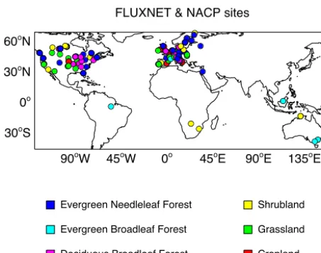
Figure 1. Distribution of 145 sites from the FLUXNET and the
North American Carbon Program (NACP) network. The duplicated sites have been removed. The color indicates different plant func-tional types (PFTs) as evergreen needleleaf forest (ENF, blue), ev-ergreen broadleaf forest (EBF, cyan), deciduous broadleaf forest (DBF, magenta), shrubland (SHR, yellow) grassland (GRA, green), and cropland (CRO, red). “mixed forests” are classified as ENF, “permanent wetlands”, “savannas”, and “woody savannas” as SHR. The PFT of each site is described in Table S1 in the Supplement.
2 Observational data sets for validation 2.1 Site-level measurements
To validate the YIBs model, we use eddy covariance mea-surements from 145 flux tower sites (Fig. 1), which are col-lected by the North American Carbon Program (Schaefer et al., 2012) (K. Schaefer, personal communication, 2013) and downloaded from the FLUXNET (http://fluxnet.ornl.gov) network. Among these sites, 138 are located in the North-ern Hemisphere, with 74 in Europe, 38 in the USA, and 24 in Canada (Table S1 in the Supplement). Sites on other con-tinents are limited. Most of the sites have one dominant plant functional type (PFT), including 54 sites of evergreen needle-leaf forests (ENF), 20 deciduous broadneedle-leaf forests (DBF), 9 evergreen broadleaf forests (EBF), 28 grasslands, 18 shrub-lands, and 16 croplands. We attribute sites with mixed forest to the ENF as these sites are usually at high latitudes. Each site’s data set provides hourly or half-hourly measurements of carbon fluxes, including gross primary productivity (GPP) and net ecosystem exchange (NEE), and CO2concentrations
and meteorological variables, such as surface air tempera-ture, relative humidity, wind speed, and shortwave radiation. 2.2 Global measurements
We use global tree height, leaf area index (LAI), GPP, net primary productivity (NPP), and phenology data sets to val-idate the vegetation model. Canopy height is retrieved using
2005 remote sensing data from the Geoscience Laser Altime-ter System (GLAS) aboard the ICESat satellite (Simard et al., 2011). LAI measurements for 1982–2011 are derived us-ing the normalized difference vegetation index (NDVI) from Global Inventory Modeling and Mapping Studies (GIMMS; Zhu et al., 2013). Global GPP observations of 1982–2011 are estimated based on the upscaling of FLUXNET eddy covariance data with a biosphere model (Jung et al., 2009). This product was made to reproduce a model (LPJmL, Lund– Potsdam–Jena managed Land) using the fraction of absorbed PAR simulated in LPJmL. As a comparison, we also use GPP observations of 1982–2008 derived based on FLUXNET, satellite, and meteorological observations (Jung et al., 2011), which are about 10 % lower than those of Jung et al. (2009). The NPP for 2000–2011 is derived using remote sensing data from Moderate Resolution Imaging Spectroradiometer (MODIS) (Zhao et al., 2005). We use the global retrieval of greenness onset derived from the Advanced Very High Reso-lution Radiometer (AVHRR) and the MODIS data from 1982 to 2011 (Zhang et al., 2014). All data sets are interpolated to the 1◦×1◦offline model resolution for comparisons.
3 YIBs model description 3.1 Vegetation biophysics
YIBs calculates carbon uptake for 9 PFTs: tundra, C3/C4 grass, shrubland, DBF, ENF, EBF, and C3/C4 cropland (Ta-ble 1). In the gridded large-scale model applications, each model PFT fraction in the vegetated part of each grid cell represents a single canopy. The vegetation biophysics sim-ulates C3 and C4 photosynthesis with the well-established Michaelis–Menten enzyme-kinetics scheme (Farquhar et al., 1980; von Caemmerer and Farquhar, 1981) and the stomatal conductance model of Ball and Berry (Ball et al., 1987). The total leaf photosynthesis (Atot, µmol m−2[leaf] s−1) is
lim-ited by one of three processes: (i) the capacity of the ribu-lose 1,5-bisphosphate (RuBP) carboxylase/oxygenase en-zyme (rubisco) to catalyze carbon fixation (Jc), (ii) the
ca-pacity of the Calvin cycle and the thylakoid reactions to regenerate RuBP supported by electron transport (Je), and
(iii) the capacity of starch and sucrose synthesis to regenerate inorganic phosphate for photo-phosphorylation in C3 plants and phosphoenolpyruvate (PEP) in C4 plants (Js).
Atot=min(Jc, Je, Js) (1)
TheJc,Je, andJs are parameterized as functions of
envi-ronmental variables (e.g., temperature, radiation, and CO2
concentrations) and the maximum carboxylation capacity (Vcmax, µmol m−2s−1) (Collatz et al., 1991, 1992):
Jc=
Vcmax
c
i−0∗ ci+Kc(1+Oi/Ko)
for C3 plant
Vcmax for C4 plant
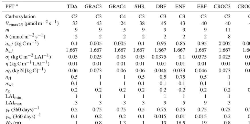
Table 1. Photosynthetic and allometric parameters for the vegetation model.
PFT∗ TDA GRAC3 GRAC4 SHR DBF ENF EBF CROC3 CROC4 Carboxylation C3 C3 C4 C3 C3 C3 C3 C3 C4
Vcmax25(µmol m−2s−1) 33 43 24 38 45 43 40 40 40
m 9 9 5 9 9 9 9 11 5
b(mmol m−2s−1) 2 2 2 2 2 2 2 8 2
awl(kg C m−2) 0.1 0.005 0.005 0.1 0.95 0.85 0.95 0.005 0.005 bwl 1.667 1.667 1.667 1.667 1.667 1.667 1.667 1.667 1.667 σl(kg C m−2LAI−1) 0.05 0.025 0.05 0.05 0.0375 0.1 0.0375 0.025 0.05 η(kg C m−1LAI−1) 0.01 0.01 0.01 0.01 0.01 0.01 0.01 0.01 0.01
n0(kg N [kg C]−1) 0.06 0.073 0.06 0.06 0.046 0.033 0.046 0.073 0.06
nrl 0.5 1 1 0.5 0.5 0.75 0.5 1 1
nwl 0.1 1 1 0.1 0.1 0.1 0.1 1 1
rg 0.2 0.2 0.2 0.2 0.2 0.2 0.2 0.2 0.2
LAImin 1 1 1 1 1 1 1 1 1
LAImax 3 3 3 3 9 5 9 3 3
γr(360 days)−1 0.5 0.75 0.75 0.5 0.75 0.25 0.75 0.75 0.75 γw(360 days)−1 0.1 0.2 0.2 0.1 0.015 0.01 0.015 0.2 0.2
H0(m) 1 0.8 1.3 1 19 16.5 19 0.8 1.3
∗Plant functional types (PFTs) are tundra (TDA), C3 grassland (GRAC3), C4 savanna/grassland (GRAC4), shrubland (SHR), deciduous broadleaf forest
(DBF), evergreen needleleaf forest (ENF), evergreen broadleaf forest (EBF), and C3/C4 cropland (CROC3/CROC4).
Je=
aleaf×PAR×α×
c
i−0∗ ci+20∗
for C3 plant
aleaf×PAR×α for C4 plant , (3)
Js= ( 0.5V
cmax for C3 plant Ks×Vcmax×
ci Ps
for C4 plant, (4)
whereciandOiare the leaf internal partial pressure (Pa) of
CO2 and oxygen, 0∗ (Pa) is the CO2 compensation point,
and Kc andKo (Pa) are Michaelis–Menten parameters for
the carboxylation and oxygenation of rubisco. The parame-tersKc,Ko, and0∗vary with temperature according to a Q10
function. PAR (µmol m−2s−1) is the incident
photosynthet-ically active radiation,aleafis leaf-specific light absorbance,
andαis intrinsic quantum efficiency.Ps is the ambient
pres-sure and Ks is a constant set to 4000 following Oleson et
al. (2010).Vcmaxis a function of the optimalVcmaxat 25◦C
(Vcmax25) based on a Q10function.
Net carbon assimilation (Anet) of leaf is given by
Anet=Atot−Rd, (5)
where Rd is the rate of dark respiration set to 0.011Vcmax
for C3 plants (Farquhar et al., 1980) and 0.025Vcmaxfor C4
plants (Clark et al., 2011). The stomatal conductance of water vapor (gsin mol [H2O] m−2s−1) is dependent on net
photo-synthesis:
gs=m
Anet×RH cs
+b, (6)
wheremandbare the slope and intercept derived from em-pirical fitting to the Ball and Berry stomatal conductance equations, RH is relative humidity, andcs is the CO2
con-centration at the leaf surface. In the model, the slopemis influenced by water stress, so that drought decreases pho-tosynthesis by affecting stomatal conductance. Appropriate photosynthesis parameters for different PFTs are taken from Friend and Kiang (2005) and the Community Land Model (Oleson et al., 2010) with updates from Bonan et al. (2011) (Table 1). In future work, we will investigate the carbon– chemistry–climate impacts of updated stomatal conductance models in YIBs (Berry et al., 2010; Pieruschka et al., 2010; Medlyn et al., 2011).
The coupled equation system of photosynthesis, stomatal conductance and CO2diffusive flux transport equations form
a cube inAnetthat is solved analytically (Baldocchi, 1994). A
simplified but realistic representation of soil water stressβis included in the vegetation biophysics following the approach of Porporato et al. (2001). The algorithm reflects the rela-tionship between soil water amount and the extent of stom-atal closure ranging from no water stress to the soil mois-ture stress onset point (s∗) through to the wilting point (swilt).
Stomatal conductance is reduced linearly between the PFT-specific values ofs∗andswiltbased on the climate model’s
soil water volumetric saturation in six soil layers (Unger et al., 2013).
as-X. Yue and N. Unger: The Yale Interactive terrestrial Biosphere model version 1.0 2403
similation respectively (Spitters et al., 1986). The leaf photo-synthesis is then integrated over all canopy layers to generate the GPP:
GPP=
LAI Z
0
AtotdL. (7)
3.2 Leaf phenology
Phenology determines the annual cycle of LAI. Plant phenol-ogy is generally controlled by temperature, water availabil-ity, and photoperiod (Richardson et al., 2013). For deciduous trees, the timing of budburst is sensitive to temperature (Vi-tasse et al., 2009) and the autumn senescence is related to both temperature and photoperiod (Delpierre et al., 2009). For small trees and grasses, such as tundra, savanna, and shrubland, phenology is controlled by temperature and/or soil moisture, depending on the species type and locations of the vegetation (Delbart and Picard, 2007; Liu et al., 2013). In the YIBs model, leaf phenology is updated on a daily basis. For the YIBs model, we build on the phenology scheme of Kim et al. (2015) and extend it based on long-term measure-ments of leaf phenology at five US sites (Yue et al., 2015a, hereinafter Y2015) and GPP at the 145 flux tower sties. A summary of the phenological parameters adopted is listed in Table 2.
3.2.1 Deciduous broadleaf forest (DBF)
We predict spring phenology of DBF using the cumulative thermal summation (White et al., 1997). The accumulative growing degree day (GDD) is calculated for thenth day from winter solstice if the 10-day average air temperature T10 is
higher than a base temperatureTb:
GDD=Xn
i=1max(T10−Tb,0) . (8)
HereTbis set to 5◦C as in Murray et al. (1989). Similar to the
approach outlined in Kim et al. (2015), the onset of greenness is triggered if the GDD exceeds a threshold valueGband a
temperature-dependent phenological factor fT is calculated
as follows:
fT =
min
1,GDD−Gb Lg
, if GDD≥Gb
0, otherwise
. (9)
Following Murray et al. (1989), the threshold Gb=a+ bexp(r×NCD) is dependent on the number of chill days (NCD), which is calculated as the total days with < 5◦C from winter solstice.
The autumn phenology is more uncertain than budburst because it is affected by both temperature and photope-riod (White et al., 1997; Delpierre et al., 2009). For the
51
0 10 20 30
ï1
ï0.5 0 0.5 1
Met
ï
GPP correlations
(a) Shrub sites (18)
0.2 0.4 0.6 0.8
ï1
ï0.5 0 0.5 1
(b) Shrub sites (18)
0 10 20 30
ï1
ï0.5 0 0.5 1
Annual mean soil temperature
Met
ï
GPP correlations
(c) Grass sites (28)
0.2 0.4 0.6 0.8
ï1
ï0.5 0 0.5 1
Annual mean soil moisture (d) Grass sites (28)
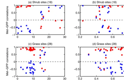
Figure 2. Correlations between monthly GPP and soil variables at (a, b) shrub and (c, d) grass sites. For each site, we calculate
corre-lation coefficients of GPP–soil temperature (red points) and GPP– soil moisture (blue squares). These correlation coefficients are then plotted against the annual mean (a, c) soil temperature (◦C) or (b,
d) soil moisture (fraction) at each site.
temperature-dependent phenology, we adopted the cumula-tive cold summation method (Dufrene et al., 2005; Richard-son et al., 2006), which calculates the accumulative falling degree day (FDD) for themth day from summer solstice as follows:
FDD=Xm
i=1min(T10−Ts,0) , (10)
whereTsis 20◦C as in Dufrene et al. (2005). Similar to the
budburst process, we determine the autumn phenological fac-tor based on a fixed thresholdFs:
fT =
max
0,1+FDD−Fs
Lf
, if FDD≤Fs
1, otherwise
. (11)
In addition, we assume photoperiod regulates leaf senescence as follows:
fP=
max
0, P−Pi Px−Pi
, ifP ≤Px
1, otherwise
, (12)
where fP is the photoperiod-limited phenology. P is day
length in minutes.Pi andPx are the lower and upper
lim-its of day length for the period of leaf fall. Finally, the au-tumn phenology of DBF is determined as the product offT
(Eq. 11) andfP (Eq. 12). Both the spring and autumn
phe-nology schemes have been evaluated with extensive ground records over the USA in Y2015.
3.2.2 Shrubland
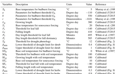
Table 2. Phenological parameters for the vegetation model.
Variables Description Units Value Reference
Tb Base temperature for budburst forcing ◦C 5 Murray et al. (1989) a Parameters for budburst thresholdGb Degree day −110 Calibrated (Y2015) b Parameters for budburst thresholdGb Degree day 550 Calibrated (Y2015) r Parameters for budburst thresholdGb Dimensionless −0.01 Murray et al. (1989) Lg Growing length Degree day 380 Calibrated (Y2015) Ts Base temperature for senescence forcing ◦C 20 Dufrene et al. (2005) Fs Threshold for leaf fall Degree day −140 Calibrated (Y2015) Lf Falling length Degree day 410 Calibrated (Y2015) Px Day length threshold for leaf fall Minutes 695 White et al. (1997) Pi Day length threshold for full dormancy Minutes 585 Calibrated (Y2015) Td Threshold for drought phenology ◦C 12 Calibrated (Fig. 2) βmin Lower threshold of drought limit for shrub Dimensionless 0.4 Calibrated (Fig. S1) βmax Upper threshold of drought limit for shrub Dimensionless 1 Calibrated (Fig. S1)
STb Base soil temperature for budburst forcing ◦C 0 White et al. (1997)
SGb Threshold for budburst with soil temperature Degree day 100 Calibrated
SLg Growing length with soil temperature Degree day 100 Calibrated
STs Base soil temperature for senescence forcing ◦C 10 Calibrated
SFs Threshold for leaf fall with soil temperature Degree day −80 Calibrated
SLf Falling length with soil temperature Degree day 100 Calibrated
βmin Lower threshold of drought limit for herbs Dimensionless 0.3 Calibrated (Fig. S1) βmax Upper threshold of drought limit for herbs Dimensionless 0.9 Calibrated (Fig. S1)
observed GPP and soil meteorology at 18 shrub sites (Fig. 2). For 10 sites with annual mean soil temperature < 9◦C, the GPP–temperature correlations are close to 1 while the GPP– moisture correlations are all negative (Fig. 2a), suggesting that temperature is the dominant phenological driver for these plants. In contrast, for eight sites with an average soil temperature > 14◦C, GPP–moisture correlations are positive and usually higher than the GPP–temperature correlations, indicating that phenology is primarily regulated by water availability at climatologically warm areas. The wide tem-perature gap (9–14◦C) is due to the limit in the availability of shrub sites. Here, we select a tentative threshold of 12◦C to distinguish cold and drought species. We also try to iden-tify phenological drivers based on soil moisture thresholds but find that both temperature- and drought-dependent phe-nology may occur at moderately dry conditions (Fig. 2b).
In the model, we apply the temperature-dependent phenol-ogyfT for shrubland if the site has annual mean soil
temper-ature < 12◦C. We use the samefT as that for DBF (Eqs. 9,
11), due to the lack of long-term phenology measurements at the shrub sites. However, if the soil temperature is > 12◦C, the plant growth is controlled by drought-limit phenologyfD
instead:
fD=
max
0, β10−βmin βmax−βmin
, ifβ10≤βmax
1, otherwise
, (13)
whereβ10is the 10-day average water stress calculated based
on soil moisture, soil ice fraction, and root fraction of each soil layer (Porporato et al., 2001). The value ofβ10 changes
from 0 to 1, with a lower value indicating drier soil. Two thresholds, βmax and βmin, represent the upper and lower
thresholds that trigger the drought limit for woody species. The values of these thresholds are set toβmax=1 andβmin=
0.4 so that the predicted phenology has the maximum corre-lations with the observed GPP seasonality (Fig. S1a in the Supplement). The shrub phenology applies for shrubland in tropical and subtropical areas, as well as tundra at the sub-arctic regions, though the phenology of the latter is usually dependent on temperature alone because the climatological soil temperature is < 12◦C.
3.2.3 Grassland
In the model, we consider temperature-dependent phenology for grassland based on soil temperature (ST) accumulation (White et al., 1997):
SGDD=Xn
i=1max(ST10−STb,0) , (14)
where ST10is the 10-day average soil temperature and STb=
0◦C. Similar to DBF, the onset of grass greenness is trig-gered if soil-temperature-based growing degree day (SGDD) is higher than a threshold value SGb(Kim et al., 2015):
fT =
min
1,SGDD−SGb
SLg
, if SGDD≥SGb
0, otherwise
, (15)
where SLg determines the grow length of grass. Both SGb
and SLg are calibrated based on observed GPP
X. Yue and N. Unger: The Yale Interactive terrestrial Biosphere model version 1.0 2405
sites is also sensitive to water stress (Fig. 2c). We apply the same drought-limit phenologyfD as shrubland (Eq. 13)
for grassland but with calibrated thresholdsβmax=0.9 and βmin=0.3 (Fig. S1b). Different from shrubland, whose
phe-nology is dominated by drought when ST > 12◦C (Fig. 2a), grassland phenology is jointly affected by temperature and soil moisture (Fig. 2c). As a result, the final phenology for grassland at warm regions is the minimum offT andfD.
3.2.4 Other PFTs
YIBs considers two evergreen PFTs, ENF at high latitudes and EBF in tropical areas. Observations do suggest that ev-ergreen trees experience seasonal changes in LAI, follow-ing temperature variations and/or water availability (Doughty and Goulden, 2008; Schuster et al., 2014). However, due to the large uncertainty of evergreen phenology, we set a con-stant phenology factor of 1.0 for these species, following the approach adopted in other process-based vegetation models (Bonan et al., 2003; Sitch et al., 2003). We implement a pa-rameterization for the impact of cold temperature (frost hard-ening) on the maximum carboxylation capacity (Vcmax) so as
to reduce cold injury for ENF during winter (Hanninen and Kramer, 2007). EBF may experience reduced photosynthesis during the dry season through the effects of water stress on stomatal conductance (Jones et al., 2014).
Crop phenology depends on planting and harvesting dates. In YIBs, we apply a global data set of crop planting and har-vesting dates (Sacks et al., 2010; Unger et al., 2013). Crop budburst occurs at the planting date and the crop continues to grow for a period of 30 days until reaching full maturity (f =1). The crop leaves begin to fall 15 days prior to the harvest date, after which phenology is set to 0. A similar treatment has been adopted in the CLM (Community Land Model; Bonan et al., 2003). Thus, crop productivity but not crop phenology is sensitive to the imposed meteorological forcings.
3.3 Carbon allocation
We adopt the autotrophic respiration and carbon allocation scheme applied in the dynamic global vegetation model (DGVM) TRIFFID (Cox, 2001; Clark et al., 2011). On a daily basis, the plant LAI is updated as follows:
LAI=f×LAIb, (16)
wheref is the phenological factor, and LAIbis the
biomass-balanced (or available maximum) LAI related to tree height. LAIb is dependent on the vegetation carbon content Cveg,
which is the sum of carbon from leaf (Cl), root (Cr), and
stem (Cw):
Cveg=Cl+Cr+Cw, (17)
where each carbon component is a function of LAIb:
Cl=σl×LAI, (18a)
Cr=σl×LAIb, (18b)
Cw=awl×LAIbbwl. (18c)
Hereσl is the specific leaf carbon density.awl andbwl are
PFT-specified allometric parameters (Table 1). The vegeta-tion carbon contentCveg is updated every 10 days based on
the carbon balance of assimilation, respiration, and litter fall. dCveg
dt =(1−λ)×NPP−3l (19)
The NPP is the net carbon uptake:
NPP=GPP−Ra. (20)
Here GPP is the total photosynthesis rate integrated over LAI. Autotrophic respiration (Ra) is split into maintenance
(Ram) and growth respiration (Rag) (Clark et al., 2011):
Ra=Ram+Rag. (21)
The maintenance respiration is calculated based on nitrogen content in leaf (Nl), root (Nr), and stem (Nw) as follows: Ram=0.012Rd
β+Nr+Nw
Nl
. (22)
where Rd is the dark respiration of leaf, which is
de-pendent on leaf temperature and is integrated over whole canopy LAI. The factor of 0.012 is the unit conversion (from mol CO2m−2s−1to kg C m−2s−1) andβis water stress
rep-resenting soil water availability. The nitrogen contents are given by
Nl=n0×Cl, (23a)
Nr=nrl×n0×Cr, (23b)
Nw=nwl×n0×η×H×LAI. (23c)
Heren0is leaf nitrogen concentration,nrlandnwlare ratios
of nitrogen concentrations of root and stem to leaves, ηis a factor scaling live stem mass to LAI and tree height H. We adopt the same values ofn0,nrl,nwl and ηas that of
the TRIFFID model (Table 1) except that nrl is set to 0.5
following observations of deciduous trees by Sugiura and Tateno (2011). The growth respiration is dependent on the residual between GPP andRambased on a ratiorgset to 0.2
for all PFTs (Knorr, 2000):
Rag=rg×(GPP−Ram) . (24)
Theλin Eq. (19) is a partitioning coefficient determining the fraction of NPP used for spreading:
λ=
1, if LAIb>LAImax
LAIb−LAImin
LAImax−LAImin
, if LAImin≤LAIb≤LAImax
0, if LAIb<LAImin
(25) where LAIminand LAImaxare minimum and maximum LAI
values for a specific PFT (Table 1). In the current model ver-sion, we turn off the fractional changes by omitting λNPP in the carbon allocation but feeding it as input for the soil respiration. The litter fall rate3lin Eq. (19) consists of
con-tributions from leaf, root, and stem as follows:
3l=γl×Cl+γr×Cr+γw×Cw. (26)
Hereγl,γr, andγware turnover rate (year−1) for leaf, root,
and stem carbon respectively. The leaf turnover rate is calcu-lated based on the phenology change every day. The root and stem turnover rates are PFT-specific constants (Table 1), de-rived based on the meta-analysis by Gill and Jackson (2000) for root and Stephenson and van Mantgem (2005) for stem. 3.4 Soil respiration
The soil respiration scheme is developed based on the CASA model (Potter et al., 1993; Schaefer et al., 2008), which con-siders carbon flows among 12 biogeochemical pools. Three live pools, including leafCl, rootCr, and woodCw, contain
biomass carbon assimilated from photosynthesis. Litterfall from live pools decomposes and transits in nine dead pools, which consist of one coarse woody debris (CWD) pool, three surface pools, and five soil pools. The CWD pool is com-posed of dead trees and woody roots. Both surface and soil have identical pools, namely structural, metabolic, and mi-crobial pools, which are distinguished by the content and functions. The structural pool contains lignin, the metabolic pool contains labile substrates, and the microbial pool rep-resents microbial populations. The remaining two soil pools, the slow and passive pools, consist of organic material that decays slowly. The full list of carbon flows among different pools has been illustrated by Schaefer et al. (2008) (cf. their Fig. 1).
When carbon transfers from poolj to pooli, the carbon loss of poolj is
Lj2i=fj2ikjCj, (27)
whereCj is the carbon in poolj,kj is the total carbon loss
rate of pool j, andfj2i is the fraction of carbon lost from
poolj transferred to pooli. The coefficientkj is dependent
on soil temperature, moisture, and texture. Meanwhile, the carbon gain of pooliis,
Gj2i =ej2i×Lj2i=ej2ifj2ikjCj, (28)
whereej2iis the ratio of carbon received by poolito the total
carbon transferred from pool j. The rest of the transferred carbon is lost due to heterotrophic respiration:
Rj2i= 1−ej2i
×Lj2i. (29)
As a result, the carbon in theith pool is calculated as dCi
dt = n X
j=1 Gj2i−
m X
k=1
Li2k. (30)
The total heterotrophic respiration (Rh) is the summation of Rj2ifor all pair pools where carbon transitions occur. The
to-tal soil carbon is the summation of carbon for all dead pools:
Csoil= 9 X
i=1
Ci. (31)
The net ecosystem productivity (NEP) is calculated as NEP= −NEE=NPP−Rh=GPP−Ra−Rh, (32)
where NEE is the net ecosystem exchange, representing net carbon flow from land to atmosphere. YIBs does not yet ac-count for NEE perturbations due to dynamic disturbance. 3.5 Ozone vegetation damage effects
We apply the semi-mechanistic parameterization proposed by Sitch et al. (2007) to account for ozone damage to pho-tosynthesis through stomatal uptake. The scheme simulates associated changes in both photosynthetic rate and stomatal conductance. When photosynthesis is inhibited by ozone, stomatal conductance decreases accordingly to resist more ozone molecules. We employed an offline regional version of YIBs to show that present-day ozone damage decreases GPP by 4–8 % on average in the eastern USA and leads to larger decreases of 11–17 % in east coast hotspots (Yue and Unger, 2014). In the current model version, the photosyn-thesis and stomatal conductance responses to ozone damage are coupled. In future work, we will update the ozone veg-etation damage function in YIBs to account for decoupled photosynthesis and stomatal conductance responses based on recent extensive metadata analyses (Wittig et al., 2007; Lom-bardozzi et al., 2013).
3.6 BVOC emissions
YIBs incorporates two independent leaf-level isoprene emis-sion schemes embedded within the exact same host model framework (Zheng et al., 2015). The photosynthesis-based isoprene scheme simulates emission as a function of the elec-tron transport-limited photosynthesis rate (Je, Eq. 3), canopy
temperature, intercellular CO2 (ci) and 0∗ (Arneth et al.,
2007; Unger et al., 2013). The MEGAN (Model of Emis-sions of Gases and Aerosols from Nature) scheme applies the commonly used leaf-level functions of light and canopy temperature (Guenther et al., 1993, 1995, 2012). Both iso-prene schemes account for atmospheric CO2sensitivity
X. Yue and N. Unger: The Yale Interactive terrestrial Biosphere model version 1.0 2407
et al., 2013). The CO2sensitivity is higher under lower
atmo-spheric CO2levels than at present day. Leaf-level
monoter-pene emissions are simulated using a simplified temperature-dependent algorithm (Lathière et al., 2006). The leaf-level isoprene and monoterpene emissions are integrated over the multiple canopy layers in the exact same way as GPP to ob-tain the total canopy-level emissions.
3.7 Implementation of YIBs into NASA ModelE2 (NASA ModelE2-YIBs)
NASA ModelE2 has a spatial resolution of 2◦×2.5◦latitude by longitude with 40 vertical levels extending to 0.1 hPa. In the online configuration, the global climate model provides the meteorological drivers to YIBs and the land-surface hy-drology submodel provides the soil characteristics (Rosen-zweig and Abramopoulos, 1997; Schmidt et al., 2014). Re-cent relevant updates to NASA ModelE2 include a dy-namic fire activity parameterization from Pechony and Shin-dell (2009) and climate-sensitive soil NOx emissions based
on Yienger and Levy (1995) (Unger and Yue, 2014). Without the YIBs implementation, the default NASA ModelE2 com-putes dry deposition using fixed LAI and vegetation cover fields from Olson et al. (2001), which are different from the climate model’s vegetation scheme (Shindell et al., 2013b). With YIBs embedded in NASA ModelE2, the YIBs model provides the vegetation cover and LAI for the dry deposi-tion scheme. The online-simulated atmospheric ozone and aerosol concentrations influence terrestrial carbon assimila-tion and stomatal conductance at the 30 min integraassimila-tion time step. In turn, the online vegetation properties, and water, en-ergy and BVOC fluxes affect air quality, meteorology and the atmospheric chemical composition. The model simulates the interactive deposition of inorganic and organic nitrogen to the terrestrial biosphere. However, the YIBs biosphere cur-rently applies fixed nitrogen levels and does not yet account for the dynamic interactions between the carbon and nitrogen cycles, and the consequences for carbon assimilation, which are highly uncertain (e.g., Thornton et al., 2007; Koven et al., 2013; Thomas et al., 2013; Zaehle et al., 2014; Houlton et al., 2015).
4 Model setup and simulations 4.1 Site-level simulations (YIBs-site)
We perform site-level simulations with the offline YIBs model at 145 eddy covariance flux tower sites for the cor-responding PFTs (Fig. 1). Hourly in situ measurements of meteorology (Sect. 2.1) are used as input for the model. We gap-filled missing measurements with the Global Modeling and Assimilation Office (GMAO) Modern Era-Retrospective Analysis (MERRA) reanalysis (Rienecker et al., 2011), as described in Yue and Unger (2014). All grasslands and most croplands are considered as C3 plants, except for some
sites where corn is grown. Meteorological measurements are available for a wide range of time periods across the differ-ent sites ranging from the minimum of 1 year at some sites (e.g., BE-Jal) to the maximum of 16 years at Harvard Forest (US-HA1). The soil carbon pool initial conditions at each site are provided by the 140-year spinup procedure using YIBs-offline (Supplement). An additional 30-year spinup is con-ducted for each site-level simulation using the initial height
H0 for corresponding PFT (Table 1) and the fixed
meteo-rology and CO2conditions at the first year of observations.
Then, the simulation is continued with year-to-year forcings at the specific site for the rest of the measurement period. For all grass and shrub sites, two simulations are performed. One applies additional drought controls on phenology as de-scribed in Sects. 3.2.2 and 3.2.3, while the other uses only temperature-dependent phenology. By comparing results of these two simulations, we assess the role of drought phenol-ogy for plants in arid and semi-arid regions.
4.2 Global offline simulation (YIBs-offline)
The global offline YIBs applies the CLM land cover data set (Oleson et al., 2010). Land cover is derived based on re-trievals from both MODIS (Hansen et al., 2003) and AVHRR (Defries et al., 2000). Fractions of 16 PFTs are aggregated into 9 model PFTs (Table 1). The soil carbon pool and tree height initial conditions are provided by the 140-year spinup procedure using YIBs-offline (Supplement). The global of-fline YIBs model is driven with WFDEI meteorology (Wee-don et al., 2014) at 1◦×1◦horizontal resolution for the pe-riod of 1980–2011. Observed atmospheric CO2
concentra-tions are adopted from the fifth assessment report (AR5) of the Intergovernmental Panel on Climate Change (IPCC; Meinshausen et al., 2011). We evaluate the simulated long-term 1980–2011 average tree height/LAI and carbon fluxes with available observations and recent multimodel intercom-parisons. Attribution of the decadal trends in terrestrial car-bon fluxes are explored in a separate follow-on companion study (Yue et al., 2015b).
4.3 Global online simulation in NASA ModelE2-YIBs
The global land cover data is identical to that used in YIBs-offline (Sect. 4.2) based on the CLM cover. Because our major research goal is to study short-term (seasonal, an-nual, decadal) interactions between vegetation physiology and atmospheric chemistry, we elect to prescribe the PFT distribution in different climatic states. We perform an on-line atmosphere-only simulation representative of the present day (∼2000s) climatology by prescribing fixed monthly-average sea surface temperature (SST) and sea ice temper-ature for the 1996–2005 decade from the Hadley Center as the boundary conditions (Rayner et al., 2006). Atmospheric CO2 concentration is fixed at the level of the year 2000
soil carbon pools and tree heights are provided by the 140-year spinup process described in the Supplement using YIBs-offline but for year 2000 (not 1980) fixed WFDEI meteorol-ogy and atmospheric CO2conditions. The NASA
ModelE2-YIBs global carbon–chemistry–climate model is run for an additional 30 model years. The first 20 years are discarded as the online spinup and the last 10-year results are aver-aged for the analyses including comparisons with observa-tions and the YIBs-offline.
4.4 Ozone vegetation damage simulation (YIBs-ozone) We perform two simulations to quantify ozone vegetation damage with the offline YIBs model based on the high and low ozone sensitivity parameterizations (Sitch et al., 2007). Similar to the setup in Yue and Unger (2014), we use of-fline hourly surface ozone concentrations simulated with the NASA ModelE2 based on the climatology and precursor emissions of the year 2000 (Sect. 4.3). In this way, atmo-spheric ozone photosynthesis damage affects plant growth, including changes in tree height and LAI. We compare the simulated ozone damage effects with the previous results in Yue and Unger (2014) that used prescribed LAI. For this up-dated assessment, we do not isolate possible feedbacks from the resultant land carbon cycle changes to the surface ozone concentrations themselves, for instance through concomitant changes to BVOC emissions and water fluxes. The impor-tance of these feedbacks will be quantified in future research using the online NASA ModelE2-YIBs framework.
5 Results
5.1 Site-level evaluation
The simulated monthly-average GPP is compared with mea-surements at 145 sites for different PFTs (Fig. 3). GPP sim-ulation biases range from −19 to 7 % depending on PFT. The highest correlation of 0.86 is achieved for DBF, mainly contributed by the reasonable phenology simulated at these sites (Fig. S2). The correlation is also high for ENF sites even though phenology is set to a constant value of 1.0. A relatively low correlation of 0.65 is modeled for EBF sites (Fig. S2). However, the site-specific evaluation shows that the simulations reasonably capture the observed magnitude and seasonality, including the minimum GPP in summer due to drought at some sites (e.g., FR-Pue and IT-Lec). Predic-tions at crop sites achieve a medium correlation of 0.77, because the prescribed crop phenology based on the plant-ing and harvestplant-ing dates data set matches reality for most sites with some exceptions (e.g., CH-Oe2). Measured GPP at shrub and grass sites show varied seasonality. For most sites, the maximum carbon fluxes are measured in the hemispheric summer season. However, for sites with arid or Mediter-ranean climate, the summer GPP is usually the lowest dur-ing the year (e.g., ES-LMa and US-Var in Fig. S2) while the
Figure 3. Comparison between observed and simulated monthly
GPP (in g C m−2day−1) from FLUXNET and NACP networks grouped by PFTs. Each point represents the average value of 1 month at one site. The red lines indicate linear regression between observations and simulations. The regression fit, correlation coef-ficient, and relative bias are shown on each panel. The PFTs in-clude evergreen needleleaf forest (ENF), evergreen broadleaf forest (EBF), deciduous broadleaf forest (DBF), shrubland (SHR), grass-land (GRA), and cropgrass-land (CRO). The detailed comparison for each site is shown in Fig. S2.
peak flux is observed during the wet season when the climate is cooler and moister. Implementing the drought-dependent phenology helps improve the GPP seasonality and decrease the root-mean-square error (RMSE) at most warm climate shrub and grass sites (Fig. S3).
A synthesis of the site-level evaluation is presented in Fig. 4. Among the 145 sites, 121 have correlations higher than 0.8 for the GPP simulation (Fig. 4a). Predictions are better for PFTs with larger seasonal variations. For exam-ple, high correlations of > 0.8 are achieved at 95 % for the ENF and DBF sites, but only 70 % for grass and 45 % for EBF sites. Low relative biases (−33 to 50 %) are achieved at 94 sites (Fig. 4b). For most PFTs, a similar fraction (65 %) of the sites have low biases falling into that range, except for cropland, where only seven sites (45 %) have the low bi-ases. The RMSE is lower than 3 g [C] day−1for 107 out of 145 sites (Fig. 4c). The highest RMSE is predicted for crop sites, where the model misses the large interannual variations due to crop rotation at some sites (e.g., BE-Lon, DE-Geb, and US-Ne2). The YIBs model performs simulations at the PFT level while measurements show large uncertainties in the carbon fluxes among biomes/species within the same PFT (Luyssaert et al., 2007). The simulated intraspecific varia-tions (in the form of standard deviation) are smaller than the measured/derived values for most PFTs (Table S2), likely be-cause of the application of fixed photosynthetic parameters for each PFT (Table 1).
sea-X. Yue and N. Unger: The Yale Interactive terrestrial Biosphere model version 1.0 2409
ï0.530 0 0.2 0.4 0.6 0.8 0.98 20
40
60 (d) Correlations for NEE
Number of sites
ï02 ï1ï0.5 0 0.5 1 4 20
40
60(e) Absolute biases in NEE (g C/day)
0.6 1 1.5 2 3 4 5
0 20 40
60 (f) RMSE of NEE (g C/day)
ï0.170 0 0.6 0.8 0.9 0.95 1 20
40 60
Number of sites
(a) Correlations for GPP
ENF EBF DBF SHR GRA CRO
ï920 ï50ï33 0 50 100 496
20 40
60(b) Relative Biases in GPP (%)
1 2 3 4 5 6 8
0 20 40
60 (c) RMSE of GPP (g C/day)
Figure 4. Bar charts of (a, d) correlation coefficients (R), (b, e) biases, and (c, f) RMSE for monthly (a–c) GPP and (d–f) NEE be-tween simulations and observations at 145 sites. Each bar represents the number of sites where theR, bias, or RMSE of simulations fall between the specific ranges as defined by thexaxis intervals. The minimum and maximum of each statistical metric are indicated as the two ends of thexaxis in the plots. The values of thexaxis are not even. The absolute biases instead of relative biases are shown for NEE because the long-term average NEE (the denominator) is usually close to zero at most sites. The PFT definitions are as in Fig. 2. Detailed comparisons at each site are shown in Figs. S2 and S4.
sonality in the observations at most sites (Fig. S4). In to-tal, 74 sites (51 %) have correlation coefficients higher than 0.6 (Fig. 4d) and 75 sites (52 %) have absolute biases within ±0.5 g [C] day−1 (Fig. 4e). For most ENF sites, the maxi-mum net carbon uptake (the minimaxi-mum NEE) is observed in spring or early summer, when GPP begins to increase while soil respiration is still at a low rate due to the cool and wet conditions (e.g., CA-Ojp and ES-ES1). Compared with other PFTs, the DBF trees usually have larger seasonality with the NEE peak in the early summer. Such seasonality helps pro-mote correlations between model and measurements, result-ing in highR(> 0.8) for 17 out of 20 sites (Fig. 4d). For shrub and grass sites, the observed seasonality of NEE is not reg-ular, though most show maximum carbon uptake in spring or early summer. Implementation of drought-dependent phe-nology helps improve the simulated NEE seasonality at some sites of these PFTs (e.g., ES-LMa and IT-Pia); however, such improvement is limited for others (Fig. S4). Simulated crop NEE reaches its maximum magnitude in summer at most sites, consistent with observations, leading to a highR(> 0.8) in 10 out 16 sites (Fig. 4d). The RMSE of simulated NEE is larger for crops relative to other PFTs because the model does not treat crop rotation (Fig. 4f).
5.2 Evaluation of YIBs-offline
YIBs-offline forced with WFDEI meteorology simulates rea-sonable spatial distributions for tree height, LAI, and GPP, all of which show maximums in the tropical rainforest biome and medium values in the Northern Hemisphere high lati-tudes (Fig. 5). Compared with the satellite observations, the
(a) Simulated height (5.1 m)
0 5 10 15 20 25 30
(b) 6height: Model - Obs (-2.1 m)
-15 -10 -5 0 5 10 15
(c) Simulated LAI (1.1 m2 m-2)
0 1 2 3 4 5 6
(d) 6LAI: Model - Obs ( 0.0 m2 m-2)
-3 -2 -1 0 1 2 3
(e) Simulated GPP (2.2 g m-2 day-1)
0 2 4 6 8 10 12
(f) 6GPP: Model - Obs (-0.1 g m-2 day-1)
-6 -4 -2 0 2 4 6
Figure 5. Simulated (a) tree height, (c) LAI, and (e) GPP and their
differences relative to observations (b, d, f). GPP data set is from Jung et al. (2009). Simulations are performed with WFDEI reanaly-sis. Statistics are the annual average for the period 1982–2011. The boxes in panel (a) represent six regions used for seasonal compari-son in Fig. 6.
simulated height is underestimated by 30 % on the annual and global mean basis (Fig. 5b). Regionally, the prediction is larger by only 4 % for tropical rainforest and temperate DBF, but by 27 % for boreal ENF, for which the model assumes a constant phenology of 1.0 all the year round. However, for the vast areas covered with grass and shrub PFTs, the sim-ulated height is lower by 41 % with maximum underestima-tion in eastern Siberia, where the model land is covered by short tundra. The modeled LAI is remarkably close to ob-servations on the annual and global mean basis (Fig. 5c, d). However, there are substantial regional biases in model LAI. Model LAI prediction is higher by 0.8 m2m−2(70 %) for bo-real ENF and by 0.1 m2m−2(5 %) for tropical rainforest. In
contrast, the simulation underestimates LAI of tropical C4 grass by 0.4 m2m−2 (30 %) and shrubland by 0.2 m2m−2
(30 %). The GPP simulation is lower than the FLUXNET-derived value by 5 % on the global scale, which is contributed by the minor underestimation for all PFTs except for tropical rainforest, where model predicts 9 % higher GPP than obser-vations (Fig. 5f).
sea-2410 X. Yue and N. Unger: The Yale Interactive terrestrial Biosphere model version 1.0
0 5 10 15 20
Obs. Height (m) 0
5 10 15 20
Model Height (m)
(a)
0 1 2 3 4
Obs. LAI (m2
m-2
) 0
1 2 3 4
Model LAI (m
2 m -2)
(b)
Amazon North America Central Africa
Europe East Asia Indonesia
Winter Spring Summer Autumn
0 2 4 6 8
Obs. GPP (g m-2 day-1)
0 2 4 6 8
Model GPP (g m
-2 day -1) (c)
0 1 2 3 4
Obs. NPP (g m-2 day-1)
0 1 2 3 4
Model NPP (g m
-2 day -1) (d)
Figure 6. Comparison of annual (a) tree height and seasonal (b) LAI, (c) GPP, and (d) (NPP between simulations and
observa-tions for the six regions shown in Fig. 5a. GPP data set is from Jung et al. (2009). Values at different regions are marked using different symbols, with distinct colors indicating seasonal means for winter (blue, December–February), spring (green, March–May), summer (red, June–August), and autumn (magenta, September–November).
sonal variations, especially for DBF, ENF, and EBF trees. LAI, GPP, and NPP also exhibit small seasonality over trop-ical areas, such as the Amazon, central Africa, and Indone-sia. However, for temperate areas, such as North America, Europe and east Asia, these variables show large seasonal variations with a minimum in winter and maximum in sum-mer. The LAI is overestimated by 20 % in the Amazon during the December-January-February season but underestimated by 25 % in Indonesia during summer (Fig. 6b). For GPP and NPP, the positive bias in Indonesia is even larger at 45 % dur-ing summer (Fig. 6c, d).
On the global scale, YIBs-offline simulates a GPP of 124.6±3.3 Pg C a−1 and NEE of −2.5±0.7 Pg C a−1 for 1982–2011. These values are consistent with estimates up-scaled from the FLUXNET observations (Jung et al., 2009, 2011; Friedlingstein et al., 2010) and simulations from 10 other carbon cycle models (Piao et al., 2013) (Fig. 7). The net biome productivity (NBP) is in opposite sign to NEE. Tropical areas (23◦S–23◦N) account for 63 % of the global GPP, including 27 % from the Amazon rainforest, 21 % from central Africa, and 5 % from Indonesia forest (Table 3). A lower contribution of 57 % from the tropics is predicted for both NPP and heterotrophic respiration. However, for NEE,
SDGVM LPJïGUESS
OCN
VEGAS LPJ
TRIFFID
CLM4CN HYLANDORCHIDE
CLM4C YIBsïoffline
ModelE2ïYIBs
GPP (Pg aï1)
NBP (Pg a
ï
1)
JU09
JU11
RLS
100 110 120 130 140 150 160
ï1 0 1 2 3 4 5
Figure 7. Comparison of simulated global GPP and net biome
pro-ductivity (NBP) from (red) YIBs-offline and (blue) ModelE2-YIBs models with 10 other carbon cycle models for 1982–2008. Each black symbol represents an independent model as summarized in Piao et al. (2013). Error bars indicate the standard deviations for in-terannual variability. The gray shading represents the global resid-ual land sink (RLS) calculated in Friedlingstein et al. (2010). The green line at the top represents the range of GPP for 1982–2008 es-timated by Jung et al. (2011) and the magenta line represents GPP for 1982–2011 from Jung et al. (2009).
only 40 % of the land carbon sink is contributed by tropical forests and grasslands, while 56 % is from temperate forests and grasslands in North America, Europe, and east Asia.
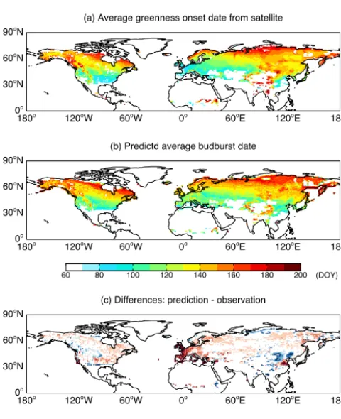
We compare the simulated budburst dates with observa-tions from satellite retrieval (Fig. 8). The model captures the basic spatial pattern of spring phenology with earlier to later budburst dates from lower to higher latitudes. On average, the observed budburst date in the Northern Hemi-sphere is DOY 133 (13 May) and the simulated is DOY 132 (12 May). Such close estimate results from the regional delay of 10 days (DOY 119 vs. 129) in Europe and advance of 4 days (DOY 140 vs. 136) in east Asia. In Y2015, ex-tensive (∼75 000 records) ground-based measurements have been used to validate the simulated spring and autumn phe-nology in the USA and both the spatial distribution and in-terannual variation of the simulation are reasonable.
5.3 Evaluation of NASA ModelE2-YIBs
con-X. Yue and N. Unger: The Yale Interactive terrestrial Biosphere model version 1.0 2411
Table 3. Summary of carbon fluxes and ozone vegetation damage in different domains and for the tropics (23◦S–23◦N).
Regions Amazon North America Central Africa Europe East Asia Indonesia Tropics Global GPP (Pg C a−1) 33.4 12.3 25.7 11.5 17.9 6.7 77.9 124.6 NPP (Pg C a−1) 15.5 7.5 12.1 7.3 10.3 2.9 36.8 65 NEE (Pg C a−1) −0.4 −0.5 −0.3 −0.4 −0.5 −0.1 −1.0 −2.5 Ra (Pg C a−1) 17.9 4.8 13.6 4.2 7.6 3.8 41.1 59.6 Rh (Pg C a−1) 15.1 7 11.8 6.9 9.8 2.8 35.8 62.5 Low ozone damage to GPP (%) −0.9 −2.4 −1.8 −2.5 −4.3 −3 −1.7 −2.1 High ozone damage to GPP (%) −2.6 −5.8 −4.4 −6.1 −9.6 −7.3 −4.4 −5 Low ozone damage to LAI (%) −0.3 −0.5 −0.6 −0.5 −0.9 −0.8 −0.5 −0.5 High ozone damage to LAI (%) −0.8 −1.2 −1.6 −1.4 −2.4 −2.1 −1.4 −1.4
(a) Average greenness onset date from satellite
0o 30o
N 60o
N 90o
N
180o 120o
W 60o
W 0o
60o
E 120o
E 180o
(b) Predictd average budburst date
0o 30o
N 60o
N 90o
N
180o 120o
W 60o
W 0o
60o
E 120o
E 180o
60 80 100 120 140 160 180 200 (DOY)
(c) Differences: prediction - observation
0o 30o
N 60o
N 90o
N
180o 120o
W 60o
W 0o
60o
E 120o
E 180o
-50 -30 -10 10 30 50 (DOY)
Figure 8. Comparison of simulated budburst dates in the
North-ern Hemisphere with remote sensing. Simulated phenology in each grid square is the composite result from DBF, tundra, shrubland, and grassland based on PFT fraction and LAI in that grid box. Both sim-ulations and observations are averaged for the period 1982–2011. Results for the Southern Hemisphere are not shown due to the lim-ited coverage of deciduous forests and cold grass species.
figuration is driven with the same meteorological forcings simulated by NASA ModelE2 except for one selected field from the WFDEI reanalysis. We found that the anomalously warmer climate over the Amazon in the global climate model (Fig. S9) causes the lower GPP in that region in NASA ModelE2-YIBs. The temperature optimum for C3 photosyn-thesis is around 30◦C, above which the maximum rate of
electron transport (Eq. 3) decreases dramatically (Farquhar et al., 1980). As a result, the higher NASA ModelE2-YIBs surface temperature in the tropical rainforest results in the lower photosynthesis rates there. With the exception of the Amazon, the NASA ModelE2-YIBs June-July-August GPP and NPP show low biases in central Africa and high latitudes in North America and Asia but high biases in Europe, west-ern USA, and eastwest-ern China (Figs. S7, S8). The sensitivity tests attribute these discrepancies to differences in canopy humidity (Fig. S11) and soil wetness (Fig. S12). Low soil wetness decreases water stressβ, reduces the slopemof the Ball–Berry equation (Eq. 6), and consequently limits photo-synthesis by declining stomatal conductance in combination with low humidity. On the global scale, the ModelE2-YIBs simulates annual GPP of 122.9 Pg C, NPP of 62 Pg C, and NEE of−2.7 Pg C, all of which are close to the YIBs-offline simulation (Table 3) and consistent with results from obser-vations and model intercomparison (Fig. 7).
5.4 Assessment of global ozone vegetation damage
2412 X. Yue and N. Unger: The Yale Interactive terrestrial Biosphere model version 1.0
(a) Low ozone damage to GPP (b) High ozone damage to GPP
-20 -16 -12 -8 -4 0 (%)
(c) Low ozone damage to LAI (d) High ozone damage to LAI
-5 -4 -3 -2 -1 0 (%)
Figure 9. Percentage of ozone vegetation damage to (top) GPP and
(bottom) LAI with (a, c) low and (b, d) high sensitivity. Both dam-ages of GPP and LAI are averaged for 1982–2011. Offline surface ozone concentrations (Fig. S5) are simulated by the GISS ModelE2 with climatology of the year 2000.
6 Conclusions and discussion
We describe and evaluate the process-based YIBs inter-active terrestrial biosphere model. YIBs is embedded into the NASA ModelE2 global chemistry–climate model and is an important urgently needed development to improve the biological realism of interactions between vegetation, atmospheric chemistry and climate. We implement both temperature- and drought-dependent phenology for DBF, shrub, and grass species. The model simulates interactive ozone vegetation damage. The YIBs model is fully validated with land carbon flux measurements from 145 ground sta-tions and global observasta-tions of canopy height, LAI, GPP, NPP, and phenology from multiple satellite retrievals.
There are several limitations in the current model setup. The vegetation parameters, Vcmax25,m, andb (Table 1) are
fixed at the PFT level, which may induce uncertainties in the simulation of carbon fluxes due to intraspecific varia-tions (Kattge et al., 2011). The model does not yet include a dynamic treatment of nitrogen and phosphorous availabil-ity because current schemes suffer from large uncertainties (Thornton et al., 2007; Zaehle et al., 2014; Houlton et al., 2015). Phenology is set to a constant value of 1 for ENF and EBF, which is not consistent with observations (O’Keefe, 2000; Jones et al., 2014). The ozone damage scheme of Sitch et al. (2007) considers coupled responses of photosynthesis and stomatal conductance while observations suggest a de-coupling (Lombardozzi et al., 2013).
Despite these limitations, the YIBs model reasonably sim-ulates global land carbon fluxes compared with both site-level flux measurements and global satellite observations.
YIBs is primed for ongoing development, for example, in-corporating community dynamics including mortality, estab-lishment, seed transport and dynamic fire disturbance (Moor-croft et al., 2001). NASA ModelE2-YIBs is available to be integrated with interactive ocean and atmospheric carbon components to offer a full global carbon–climate model, for example, for use in interpreting and diagnosing new satellite data sets of atmospheric CO2concentrations. In the current
form, NASA ModelE2-YIBs provides a useful new tool to investigate the impacts of air pollution on the carbon budget, water cycle, and surface energy balance, and, in turn, the im-pacts of changing vegetation physiology on the atmospheric chemical composition. Carbon–chemistry–climate interac-tions, a relatively new interdisciplinary research frontier, are expected to influence the evolution of Earth’s climate system on multiple spatiotemporal scales.
Code availability
The YIBs model (version 1.0) site-level source code is avail-able at https://github.com/YIBS01/YIBS_site. The source codes for the global offline and global online versions of the YIBs model (version 1.0) are available through collabora-tion. Please submit a request to X. Yue ([email protected]) and N. Unger ([email protected]). Auxiliary forcing data and related input files must be obtained independently.
The Supplement related to this article is available online at doi:10.5194/gmd-8-2399-2015-supplement.
Acknowledgements. Funding support for this research is provided
by the NASA Atmospheric Composition Campaign Data Analysis and Modeling Program. This project was supported in part by the facilities and staff of the Yale University Faculty of Arts and Sciences High Performance Computing Center. We are grateful to Y. Kim, I. Aleinov, and N. Y. Kiang for access to unpublished codes. We thank Ranga B. Myneni and Zaichun Zhu for providing the AVHRR LAI3g data set.
Edited by: J. Williams
References
Ainsworth, E. A., Yendrek, C. R., Sitch, S., Collins, W. J., and Em-berson, L. D.: The effects of tropospheric ozone on net primary productivity and implications for climate change, Annu. Rev. Plant Biol., 63, 637–661, doi:10.1146/Annurev-Arplant-042110-103829, 2012.
X. Yue and N. Unger: The Yale Interactive terrestrial Biosphere model version 1.0 2413
Baldocchi, D.: An Analytical Solution for Coupled Leaf Photo-synthesis and Stomatal Conductance Models, Tree Physiol., 14, 1069–1079, 1994.
Ball, J. T., Woodrow, I. E., and Berry, J. A.: A model predicting stomatal conductance and its contribution to the control of photo-synthesis under different environmental conditions, in: Progress in Photosynthesis Research, edited by: Biggins, J., Nijhoff, Dor-drecht, the Netherlands, 221–224, 1987.
Beer, C., Reichstein, M., Tomelleri, E., Ciais, P., Jung, M., Carval-hais, N., Rodenbeck, C., Arain, M. A., Baldocchi, D., Bonan, G. B., Bondeau, A., Cescatti, A., Lasslop, G., Lindroth, A., Lomas, M., Luyssaert, S., Margolis, H., Oleson, K. W., Roupsard, O., Veenendaal, E., Viovy, N., Williams, C., Woodward, F. I., and Pa-pale, D.: Terrestrial Gross Carbon Dioxide Uptake: Global Dis-tribution and Covariation with Climate, Science, 329, 834–838, doi:10.1126/Science.1184984, 2010.
Berry, J. A., Beerling, D. J., and Franks, P. J.: Stomata: key players in the earth system, past and present, Curr. Opin. Plant Biol., 13, 233–240, doi:10.1016/J.Pbi.2010.04.013, 2010.
Bonan, G. B., Levis, S., Sitch, S., Vertenstein, M., and Oleson, K. W.: A dynamic global vegetation model for use with climate models: concepts and description of simulated vegetation dy-namics, Glob. Change Biol., 9, 1543–1566, doi:10.1046/J.1365-2486.2003.00681.X, 2003.
Bonan, G. B., Lawrence, P. J., Oleson, K. W., Levis, S., Jung, M., Reichstein, M., Lawrence, D. M., and Swenson, S. C.: Improving canopy processes in the Community Land Model version 4 (CLM4) using global flux fields empirically in-ferred from FLUXNET data, J. Geophys. Res., 116, G02014, doi:10.1029/2010jg001593, 2011.
Clark, D. B., Mercado, L. M., Sitch, S., Jones, C. D., Gedney, N., Best, M. J., Pryor, M., Rooney, G. G., Essery, R. L. H., Blyth, E., Boucher, O., Harding, R. J., Huntingford, C., and Cox, P. M.: The Joint UK Land Environment Simulator (JULES), model descrip-tion – Part 2: Carbon fluxes and vegetadescrip-tion dynamics, Geosci. Model Dev., 4, 701–722, doi:10.5194/gmd-4-701-2011, 2011. Collatz, G. J., Ball, J. T., Grivet, C., and Berry, J. A.:
Physio-logical and Environmental-Regulation of Stomatal Conductance, Photosynthesis and Transpiration – a Model That Includes a Laminar Boundary-Layer, Agr. Forest Meteorol., 54, 107–136, doi:10.1016/0168-1923(91)90002-8, 1991.
Collatz, G. J., Ribas-Carbo, M., and Berry, J. A.: Coupled Photosynthesis-Stomatal Conductance Model for Leaves of C4 Plants, Aust. J. Plant Physiol., 19, 519–538, 1992.
Cox, P. M.: Description of the “TRIFFID” Dynamic Global Vegeta-tion Model, Hadley Centre, Technical Note 24, Berks, UK, 2001. Defries, R. S., Hansen, M. C., Townshend, J. R. G., Janetos, A. C., and Loveland, T. R.: A new global 1-km dataset of percentage tree cover derived from remote sensing, Glob. Change Biol., 6, 247–254, doi:10.1046/J.1365-2486.2000.00296.X, 2000. Delbart, N. and Picard, G.: Modeling the date of leaf
appear-ance in low-arctic tundra, Glob. Change Biol., 13, 2551–2562, doi:10.1111/J.1365-2486.2007.01466.X, 2007.
Delpierre, N., Dufrene, E., Soudani, K., Ulrich, E., Cecchini, S., Boe, J., and Francois, C.: Modelling interannual and spa-tial variability of leaf senescence for three deciduous tree species in France, Agr. Forest Meteorol., 149, 938–948, doi:10.1016/J.Agrformet.2008.11.014, 2009.
Doughty, C. E. and Goulden, M. L.: Seasonal patterns of tropical forest leaf area index and CO2exchange, J. Geophys. Res., 113,
G00b06, doi:10.1029/2007jg000590, 2008.
Dufrene, E., Davi, H., Francois, C., le Maire, G., Le Dan-tec, V., and Granier, A.: Modelling carbon and water cy-cles in a beech forest Part I: Model description and uncer-tainty analysis on modelled NEE, Ecol. Model, 185, 407–436, doi:10.1016/J.Ecolmodel.2005.01.004, 2005.
Farquhar, G. D., Caemmerer, S. V., and Berry, J. A.: A Biochemical-Model of Photosynthetic Co2 Assimilation in Leaves of C-3 Species, Planta, 149, 78–90, doi:10.1007/Bf00386231, 1980. Friedlingstein, P., Cox, P., Betts, R., Bopp, L., Von Bloh, W.,
Brovkin, V., Cadule, P., Doney, S., Eby, M., Fung, I., Bala, G., John, J., Jones, C., Joos, F., Kato, T., Kawamiya, M., Knorr, W., Lindsay, K., Matthews, H. D., Raddatz, T., Rayner, P., Reick, C., Roeckner, E., Schnitzler, K. G., Schnur, R., Strassmann, K., Weaver, A. J., Yoshikawa, C., and Zeng, N.: Climate-carbon cy-cle feedback analysis: Results from the (CMIP)-M-4 model inter-comparison, J. Climate, 19, 3337–3353, doi:10.1175/Jcli3800.1, 2006.
Friedlingstein, P., Houghton, R. A., Marland, G., Hackler, J., Boden, T. A., Conway, T. J., Canadell, J. G., Raupach, M. R., Ciais, P., and Le Quere, C.: Update on CO2 emissions, Nat. Geosci., 3, 811–812, doi:10.1038/Ngeo1022, 2010.
Friedlingstein, P., Andrew, R. M., Rogelj, J., Peters, G. P., Canadell, J. G., Knutti, R., Luderer, G., Raupach, M. R., Schaeffer, M., van Vuuren, D. P., and Le Quere, C.: Persistent growth of CO2 emis-sions and implications for reaching climate targets, Nat. Geosci., 7, 709–715, doi:10.1038/Ngeo2248, 2014.
Friend, A. D. and Kiang, N. Y.: Land surface model devel-opment for the GISS GCM: Effects of improved canopy physiology on simulated climate, J. Climate, 18, 2883–2902, doi:10.1175/Jcli3425.1, 2005.
Gill, R. A. and Jackson, R. B.: Global patterns of root turnover for terrestrial ecosystems, New Phytol., 147, 13–31, doi:10.1046/J.1469-8137.2000.00681.X, 2000.
Guenther, A. B., Zimmerman, P. R., Harley, P. C., Monson, R. K., and Fall, R.: Isoprene and Monoterpene Emission Rate Variabil-ity – Model Evaluations and SensitivVariabil-ity Analyses, J. Geophys. Res., 98, 12609–12617, doi:10.1029/93jd00527, 1993.
Guenther, A. B., Hewitt, C. N., Erickson, D., Fall, R., Geron, C., Graedel, T., Harley, P., Klinger, L., Lerdau, M., Mckay, W. A., Pierce, T., Scholes, B., Steinbrecher, R., Tallamraju, R., Tay-lor, J., and Zimmerman, P.: A Global-Model of Natural Volatile Organic-Compound Emissions, J. Geophys. Res., 100, 8873– 8892, doi:10.1029/94jd02950, 1995.
Guenther, A. B., Jiang, X., Heald, C. L., Sakulyanontvittaya, T., Duhl, T., Emmons, L. K., and Wang, X.: The Model of Emissions of Gases and Aerosols from Nature version 2.1 (MEGAN2.1): an extended and updated framework for modeling biogenic emis-sions, Geosci. Model Dev., 5, 1471–1492, doi:10.5194/gmd-5-1471-2012, 2012.
Hanninen, H. and Kramer, K.: A framework for modelling the an-nual cycle of trees in boreal and temperate regions, Silva Fenn., 41, 167–205, 2007.