ON THE AVERAGE LOWER
2-DOMINATION NUMBER OF A GRAPH
T. TURACI1, §
Abstract. Computer scientists and network scientists want a speedy, reliable, and non-stop communication. In a communication network, the vulnerability measures the re-sistance of the network to disruption of operation after the failure of certain stations or communication links. The average lower 2-domination number of a graph G rela-tive to a vertex v is the cardinality of a minimum 2-dominating set in G containing
v. Consider the graphG modeling a network. The average lower 2-domination num-ber of G, denoted asγ2av(G), is a new measure of the network vulnerability, given by
γ2av(G) = |V(G)|1 P
v∈V(G)γ2v(G). In this paper, above mentioned new parameter is defined and examined, also the average lower 2-domination number of well known graph families are calculated. Then upper and lower bounds are determined and exact formulas are found for the average lower 2-domination number of any graphG.
Keywords: Graph vulnerability; Connectivity; Network design and communication; Dom-ination number; Average lower 2-domDom-ination number
AMS Subject Classification: 05C40, 05C69, 68M10, 68R10.
1. Introduction
Networks are important structures and appear in many different applications and set-tings. The most common networks are telecommunication networks, computer networks, the internet, road and rail networks and other logistic networks [20]. In a communication network, the measures of vulnerability are essential to guide the designers in choosing a suitable network topology. They have an impact on solving difficult optimization problems for networks [20]. Furthermore, the fundamental component of a distributed system is the interconnection network.
The network topology is significant since the communication between processors is de-rived via message exchange in distributed systems. For this reason, a communication network is modeled by a graph to measure the vulnerability, where stations correspond to vertices and communication links correspond to edges. The vulnerability value of a communication network shows the resistance of the network after the disruption of some centers or connection lines until a communication breakdown. As the networks begin losing connection lines or centers, eventually, there is a loss of efficiency [2, 3, 12, 19].
1 Department of Mathematics, Faculty of Science, Karabuk University 78050, Karabuk, Turkey. e-mail: [email protected], ORCID: http://orcid.org/0000-0002-6159-0935.
§ Manuscript received: July 26, 2017; accepted: January 29, 2018.
TWMS Journal of Applied and Engineering Mathematics, Vol.9, No.3 cI¸sık University, Department of Mathematics, 2019; all rights reserved.
In the literature, various measures have been defined to measure the robustness of net-work and a variety of graph theoretic parameters have been used to derive formulas to calculate network vulnerability. The graph vulnerability relates to the study of graph when some of its elements (vertices or edges) are removed. The measures of graph vulner-ability are usually invariants that measure how a deletion of one or more network elements changes properties of the network. The best known measure of reliability of a graph is its connectivity. The vertex (edge) connectivity is defined to be the minimum number of vertices (edges) whose deletion results in a disconnected or trivial graph, also it is denoted by k(G) ( k0(G) ) [14]. Then the toughness [12], the integrity [7], the residual closeness [22], the domination number [8], the bondage number [4, 5], the 2-domination number [18], the 2-bondage number [18], etc. have been proposed for measuring the vulnerability of networks. Recently, some average vulnerability parameters such as the average lower independence number [3, 10, 16], the average lower domination number [6, 16, 21], the av-erage connectivity number [9], the avav-erage lower connectivity number [1] and the avav-erage lower bondage number [23], etc. have been defined. The average parameters have been found to be more useful in some circumstance than the corresponding measures based on worst-case situation [15].
Let G = (V(G), E(G)) be a simple undirected graph of order n. For any vertex
v ∈ V(G), the open neighborhood of v is NG(v) = {u ∈ V(G)|uv ∈ E(G)} and closed neighborhood of v is NG[v] = NG(v)∪ {v}. The degree of a vertex v in G, denoted by
dG(v), is the size of its open neighborhood [13]. The minimum degree of the graphG is denoted byδ(G). A vertexv with degree one is called a leaf vertex (or a pendant vertex) and a vertex adjacent to a leaf vertex is called a support vertex. The graph G is called
r-regular graph if dG(v) =r for every vertexv ∈V(G). The distanced(u, v) between two verticesu and v in Gis the length of a shortest path between them. The diameter of G, denoted bydiam(G) is the largest distance between two vertices inV(G). A setS⊆V(G) is a dominating set if every vertex in V(G)\S is adjacent to at least one vertex in S. The minimum cardinality taken over all dominating sets of G is called the domination number ofGand it is denoted byγ(G) [13]. Another domination concept is 2-domination number. A 2-dominating set of a graphG is a set D⊆ V(G) of vertices of G such that every vertex ofV(G)\Dhas at least two neighbors inD. The 2-domination number of a graphG, denoted byγ2(G), is the minimum cardinality of a 2-dominating set of the graph
G[11, 18].
In 2004, Henning introduced the concept of average domination and average indepen-dence [16]. Finding maximum dominating sets and maximum independent sets in graphs are the problems closely related to the concept of average domination and average inde-pendence. Also, the average lower domination and the average lower independence number are the theoretical vulnerability parameters for a network which have been modeled by a graph [3, 6]. The average lower domination number of a graph G, denoted by γav(G), is defined as: γav(G) = |V(1G)|
P
v∈V(G)γv(G), where the lower domination number, denoted by γv(G), is the minimum cardinality of a dominating set of the graph G that contains the vertexv [10, 16].
The aim of this paper is to define a new vulnerability parameter, so called average lower 2-domination number. In the Section 2, well-known basic results have been given for the average lower domination number and the 2-domination number, respectively. In the Section 3, the average lower 2-domination number denoted by γ2av(G) has been defined.
2. Basic Results
In this section, well known basic results with regard to the average lower domination number and the 2-domination number are given.
Theorem 2.1. [16] If G is a graph of order n with the domination number γ(G), then
γav(G)≤γ(G) + 1−γ(nG), with equality if and only if Ghas a unique γ(G)-set.
Theorem 2.2. [16] If K1,n−1 is a star graph of order n, where n≥3 ,then
γav(K1,n−1) = 2−
1
n.
Theorem 2.3. [16] If Pn is a path graph of order n, then
γav(Pn) =
n+2 3 −
2
3n ,if n≡2 (mod3); n+2
3 ,otherwise.
Theorem 2.4. [16] If Cn is a cycle graph of order n, then γav(Cn) =dn3e. Theorem 2.5. [16] If Kn is a complete graph of order n, then γav(Kn) = 1.
Observation 2.1. If Wn is a wheel graph of order n+ 1, then γav(Wn) = 2nn+1+1. Theorem 2.6. [18] Every leaf vertex of a graph G is in everyγ2(G)-set.
Theorem 2.7. [18] If Kn is a complete graph of order n, then γ2(Kn) =min{2, n}. Theorem 2.8. [18] If Pn is a path graph of order n, then γ2(Pn) =bn2c+ 1.
Theorem 2.9. [18] If Cn is a cycle graph of order n, then γ2(Cn) =bn+12 c. Observation 2.2. If Wn is a wheel graph of order n+ 1, where n≥3, then
γ2(Wn) =
2 ,if n=3,4;
1 +dn
3e ,if n≥5.
Theorem 2.10. [13] If T is a tree of ordern, then γ2(T)≥ n+12 .
3. The Average Lower 2-domination Number
In this section, a new parameter of a graph has been introduced. It is called the average lower 2-domination number, defined by γ2av(G) = |V(1G)|Pv∈V(G)γ2v(G), where γ2v(G) is the cardinality of the minimum 2-domination set in G that contains v, called lower 2-domination number ofGrelative tov.
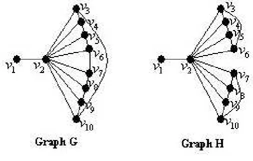
When a graph is considered as modeling a network, the average lower 2-domination number may be more sensitive to the vulnerability of a graph than the other known vulnerability measures. For example, letG and H, presented in Figure 1, be two graphs, where |V(G)| = |V(H)| = 10 and |E(G)| = |E(H)| = 17. The graphs G and H have not only equal connectivity but also equal domination number, average lower domination number and 2-domination number, respectively, k(G) = k(H) = 1, γ(G) = γ(H) = 1,
γav(G) = γav(H) = 1.9 and γ2(G) = γ2(H) = 5. These values can be checked by the
readers. So, how can be distinguished between the graphsGand H?
To compute theγ2av(H) for the graphH, the 2-dominating sets that include every vertex
vi ∈V(H) must be found. Sets {v1, v3, v5, v7, v9},{v2, v1, v4, v6, v7, v9},{v3, v1, v5, v7, v9},
{v4, v1, v6, v8, v10},{v5, v1, v3, v7, v9},{v6, v1, v4, v8, v10},{v7, v1, v3, v5, v9},{v8, v1, v4, v6, v10},
{v9, v1, v3, v5, v7}and {v10, v1, v4, v6, v8} are minimum 2- dominating sets that include
Figure 1. GraphsGand H
γ2v1(H) = 5, γ2v2(H) = 6, γ2v3(H) = 5, γ2v4(H) = 5, γ2v5(H) = 5, γ2v6(H) = 5,
γ2v7(H) = 5, γ2v8(H) = 5, γ2v9(H) = 5 andγ2v10(H) = 5. As a result, γ2av(H) = 5.1 is
obtained. The reader can check thatγ2av(G) = 5.
Thus, the average lower 2-domination number may be a better parameter than the connectivity, the domination number, the average lower domination number and the 2-domination number to distinguish these two graphs G and H. Furthermore, it is not difficult to see that the graphHis more vulnerable than the graphG. Because, if an attack occurs on the links that are relevant to the vertexv2, then two disconnected components
would be remain in the graph G, while three disconnected components would be remain in the graph H. Due to γ2av(G) < γ2av(H), it can be said that the graph H is more vulnerable than the graphG. In other words the graphG is tougher than the graphH.
4. The Upper and Lower Bounds and Exact Formulas
Theorem 4.1. Let G be any connected graph of order n. If the 2-dominating set is unique, then
γ2av(G) =γ2(G) + 1−
γ2(G)
n .
Proof. LetD∗ be unique 2-dominating set and letv1∗, v2∗, ..., v∗|D∗| be vertices ofD∗. Then
γ2v∗i(G) =γ2(G), wherei∈ {1, ...,|D∗|}is obtained. It is clear that the lower 2-domination
number isγ2(G) + 1 for every vertex of V(G)\D∗. Thus,
γ2av(G) = |V(1G)|(
P
vi∗∈D∗γ2v∗ i(G) +
P
vi∈V(G)\D∗γ2vi(G))
= |V(1G)|(|D∗|γ2(G) + (γ2(G) + 1)(|V(G)| − |D∗|))
=γ2(G) + 1− |D ∗|
|V(G)| is found.
Clearly,|D∗|=γ2(G) and |V(G)|=n. Then,
γ2av(G) =γ2(G) + 1−
γ2(G)
n
is obtained.
Theorem 4.2. If G is a connected graph of order n, then
γ2(G)≤γ2av(G)≤γ2(G) + 1−
γ2(G)
Proof. LetDbe a set including minimum 2-dominating sets. If the union of the minimum 2-dominating sets is equal toV(G), then the lower 2-domination number isγ2(G) for every
vertex of V(G). Thus, the lower bound is γ2av(G) = γ2(G). Furthermore, γ2av(G) =
γ2(G) + 1−γ2(nG) which is obtained by the Theorem 4.1 is also upper bound. As a result,
γ2(G)≤γ2av(G)≤γ2(G) + 1−γ2(nG) is obtained. Hence the proof is completed.
Theorem 4.3. Let G be any connected graph of order n, where n≥2. Then,
2≤γ2av(G)≤n−1 + 1
n.
Proof. The complete graphK2 is the smallest connected graph providing thatn≥2. Due
to γ2av(K2) = 2, a fair lower bound is obtained. On the other hand, the maximum
2-domination number isn−1 for any connected graphGof ordern. This value is obtained for the star graph K1,n−1. Since the γ2(K1,n−1)-set is unique for the graph K1,n−1, so
γ2av(K1,n−1) = n− n−n1 = n−1 + 1n is obtained by the Theorem 4.1. As a result,
2≤γ2av(G)≤n−1 +1n is obtained.
Theorem 4.4. If G is a connected graph of order nand e is an edge on the complement of G, then γ2av(G)≥γ2av(G+e).
Proof. Consider the graphG+e, obtained adding toE(G) any edgeefrom the complement ofG. It is easy to see thatγ2v(G)≥γ2v(G+e) for every vertexv∈V(G) andv∈V(G+e). It is clear that (n1)P
vV(G)γ2v(G) ≥ (n1)
P
vV(G+e)γ2v(G+e) is known. As a result,
γ2av(G)≥γ2av(G+e) is obtained.
Definition 4.1. [12]Consider two graphsG1 = (V(G1), E(G1))andG2 = (V(G2), E(G2)). The join graphG=G1+G2 is the graph G= (V(G), E(G)), such that V(G) =V(G1)∪
V(G2) and E(G) =E(G1)∪E(G2)∪ {uv|u∈V(G1), v∈V(G2)}.
Theorem 4.5. Let G and H be two connected graphs of order n and m, respectively.
(a) If γ(G) =γ(H) = 1, then 2≤γ2av(G+H)≤3−m2+n. (b) For any graphs G and H, 2≤γ2av(G+H)≤4.
Proof. For (a): Due to γ(G) = 1 and γ(H) = 1, then γ2(G+H) = 2 is obtained.
More-over, γ2(G+H)- set can be unique. Thus, γ2av(G+H) ≤ 3− m2+n is known by the Theorem 4.2. Let graphsGandH be complete graphs of ordernandm, respectively. So,
γ2av(G+H) = 2 is obtained. As a result, 2≤γ2av(G+H)≤3−m2+n.
For (b): Ifγ2(G)>2,γ2(H)>2,γ(G)>2 andγ(H)>2, then the cardinality of every
γ2v(G+H)-set is 4. So,γ2av(G+H) = 4 is obtained. It is known that 2≤γ2av(G+H) from the (a). As a result, 2≤γ2av(G+H)≤4 is obtained.
Theorem 4.6. Let G and H be two connected graphs of order n and m, respectively. If
n≥2 and m≥2, then γ2av(G) +γ2av(H)≥γ2av(G+H).
Proof. Clearly,γ2av(G)≥2 andγ2av(H)≥2 are known by the Theorem 4.3. Furthermore,
clearlyγ2av(G+H)≤4 is known by the Theorem 4.5. As a result, γ2av(G) +γ2av(H) ≥
γ2av(G+H) is obtained.
Proof. Consider a tree T of ordern. Furthermore, a set called by ST(p) is expressed by
ST(p) = {v ∈ V(T)|pv ∈ E(T)and dT(v) = 1}, where p is a support vertex. Clearly, if
|ST(p)| ≥ 2 has been got for every support vertex p, then γ2(T)-set will be an unique
set. Since the number of support vertices is s, then γ2(T) = n−s is obtained. So
γ2av(T) =n−s+ns, which this value is a lower bound, is found by the Theorem 4.1. If
|ST(p)|<2 for any support vertex, then the vertex p is not 2-dominated by the vertices of degree 1 that are neighbors of the support vertexp. Thus, the cardinality ofγ2p(T)-set
is increased. So, γ2av(T) > n−s+ ns is found. As a result, γ2av(T) ≥ n−s+ sn is
obtained.
Theorem 4.8. Let T be any connected tree of order n, then γ2av(T)≥ n+12 .
Proof. The proof follows directly from the Theorem 2.10.
5. The Average Lower 2-domination Number of Some Graphs
In this section, the average lower 2-domination numbers of the well known graph classes such asPn,Cn,Knand K1,n−1 have been calculated.
Theorem 5.1. If Pn is a path graph of order n, then
γ2av(Pn) =
(
bn
2c+ 2−
bn 2c+1
n ,if n is odd; n
2 + 1 ,if n is even.
Proof. Ifnis odd,γ2(Pn)-set is unique in the graphPn. Clearly,γ2(Pn) =bn2c+ 2− bn
2c+1
n is known by the Theorems 2.8 and 4.1, respectively. Ifnis even, thenγ2(Pn) = n2 + 1 can be written. It is clear that the lower 2-domination number is n2 + 1 for the every vertex
v∈V(Pn). Thus,γ2av(Pn) = n2 + 1 is obtained.
Theorem 5.2. If Cn is a cycle graph of order n, then γ2av(Cn) =bn+12 c.
Proof. Clearly, γ2(Cn) = bn+12 c is known by the Theorem 2.10. Since the graph Cn is regular graph, the cardinality of the γ2v(Cn)-set is bn+12 c for every vertex v ∈ V(Cn).
Thus,γ2av(Cn) =bn+12 c is obtained.
Corollary 5.1. If Kn is a complete graph of order n≥2, then γ2av(Kn) = 2.
Proof. Clearly, to obtain the 2-domination number ofKn any two vertices must be taken toγ2(Kn)−set(see Theorem 2.7.). Thus, the definition of the average lower 2-domination
number,γ2av(Kn) = 2 is obtained.
Corollary 5.2. If K1,n−1 is a star graph of order n, then γ2av(K1,n−1) =n−1 +n1. Proof. Clearly, γ2(K1,n−1) = n− 1 is known by the Theorem 2.6, Moreover, the
2-dominating set is unique. Thus, by the Theorem 4.1
γ2av(K1,n−1) =γ2(K1,n−1) + 1−
γ2(K1,n−1)
n =n−1 +
1
n
6. Conclusion
In this study, a new graph theoretical parameter namely the average lower 2-domination number has been presented for the network vulnerability. The present parameter has been constructed by summing of the lower 2-domination number of every vertex of a graph divided by the number of vertices of the graph. Additionally, the stability of popular interconnection networks has been studied and their average lower 2-domination numbers have been computed. These networks have been modeled with the complete graphs, the path graphs, the cycle graphs, the star graphs. Furthermore, upper and lower bounds and exact formulas have been obtained for the average lower 2-domination number of any graphG, the join graphG1+G2 and trees. As a further study, exact formulas or bounds
may be obtained for graph operations and large network topologies.
7. Acknowledgement
The author would like to express his deepest gratitude to the anonymous referees for the constructive suggestions and comments that has improved the quality of this paper.
References
[1] Aslan, E., (2014), The Average Lower Connectivity of Graphs, Journal of Applied Mathematics, 2014, ID:807834, 4 Pages.
[2] Ayta¸c, A. and Odabas, Z.N., (2011), Residual Closeness of Wheels and Related Networks, Interna-tional Journal of Foundations of Computer Science, 22(5), pp. 1229-1240.
[3] Ayta¸c, A. and Turaci, T., (2011), Vertex Vulnerability Parameter of Gear Graphs, International Journal of Foundations of Computer Science, 22(5), pp. 1187-1195.
[4] Ayta¸c, A., Turaci, T. and Odabas, Z.N., (2013), On The Bondage Number of Middle Graphs, Math-ematical Notes, 93(6), pp. 803-811.
[5] Ayta¸c, A., Odabas, Z.N. and Turaci, T.,(2011), The Bondage Number for Some Graphs, Comptes Rendus de Lacademie Bulgare des Sciences, 64(7), pp. 925-930.
[6] Ayta¸c, V., (2012), Average Lower Domination Number in Graphs, Comptes Rendus de Lacademie Bulgare des Sciences, 65(12), pp. 1665-1674.
[7] Barefoot, C.A., Entringer, R. and Swart, H., (1987), Vulnerability in graphs-a comparative survey, J. Combin. Math. Combin. Comput., 1, pp. 13-22.
[8] Bauer, D., Harary, F., Nieminen, J. and Suffel C. L., (1983), Domination alteration sets in graph, Discrete Math., 47, pp. 153-161.
[9] Beineke, L.W., Oellermann, O.R. and Pippert, R.E., (2002), The Average Connectivity of a Graph, Disc. Math., 252(1-3), pp. 31-45.
[10] Blidia, M., Chellali, M. and Maffray, F., (2005), On Average Lower Independence and Domination Number in Graphs, Disc. Math., 295, pp. 1-11.
[11] Chellali, M., (2006), Bounds on the 2-Domination Number in Cactus Graps, Opuscula Mathematica, 26(1), pp. 5-12.
[12] Chvatal, V., (1973), Tough graphs and Hamiltonian circuits, Discrete Math., 5, pp. 215-228.
[13] Fink, J.F. and Jacobson M.S., (1985), n-domination in graphs, in: Alavi Y. and Schwenk A. J.(eds), Graph Theory with Applications to Algorithms and Computer Science, NewYork, Wiley, pp. 283-300. [14] Frank, H. and Frisch, I.T., (1970), Analysis and design of survivable Networks, IEEE Transactions on
Communications Technology, 18(5), pp. 501-519.
[15] Henning, M.A. and Oellermann, O.R., (2004), The Average Connectivity of a Digraph, Discrete App. Math., 140(1-3), pp. 143-153.
[17] Javaid, I. and Shokat, S., (2008), On the Partition Dimension of Some Wheel Related Graphs, Journal of Prime Research in Mathematics, 4, pp. 154-164.
[18] Krzywkowski, M., (2013), 2-bondage in graphs, International Journal of Computer Mathematics, 90(7), pp. 1358-1365.
[19] Mishkovski, I., Biey, M. and Kocarev, L., (2011), Vulnerability of complex Networks, Commun. Non-linear Sci Numer Simulat., 16, pp. 341-349.
[20] Newport, K.T. and Varshney, P.K., (1991), Design of survivable communication networks under per-formance constraints, IEEE Transactions on Reliability, 40, pp. 433-440.
[21] Tuncel, G.H., Turaci, T. and Coskun, B., (2015), The Average Lower Domination Number and Some Results of Complementary Prisms and Graph Join, Journal of Advanced Research in Applied Math-ematics, 7(1), pp. 52-61.
[22] Turaci, T. and Okten, M., (2015), Vulnerability Of Mycielski Graphs via Residual Closeness, Ars Combinatoria, 118, pp. 419-427.
[23] Turaci, T., (2016), On The Average Lower Bondage Number a Graph, RAIRO-Operations Research, 50(4-5), pp. 1003-1012.