Asymptotic behavior of a system of two difference equations of exponential form

(1)

ISSN: 2008-6822 (electronic)

http://dx.doi.org/10.22075/ijnaa.2017.1301.1320

Asymptotic behavior of a system of two difference

equations of exponential form

Mai Nam Phong∗, Vu Van Khuong

Department of Mathematical Analysis, University of Transport and Communications, Hanoi City, Vietnam

(Communicated by Th.M. Rassias)

Abstract

In this paper, we study the boundedness and persistence of the solutions, the global stability of the unique positive equilibrium point and the rate of convergence of a solution that converges to the equilibrium E = (¯x, y) of the system of two difference equations of exponential form:¯

xn+1 =

a+e−(bxn+cyn)

d+bxn+cyn

, yn+1 =

a+e−(byn+cxn)

d+byn+cxn

where a, b, c, dare positive constants and the initial valuesx0, y0 are positive real values.

Keywords: Difference equations; boundedness; persistence; asymptotic behavior; rate of convergence.

2010 MSC: 39A10.

1. Introduction and preliminaries

Difference equations have many applications in applied sciences, there are many papers and books that can be found concerning the theory and applications of difference equations, see [1, 4, 6, 7] and the references cited therein. Recently, there has been a great interest in studying the qualitative properties of difference equations and systems of difference equations of exponential form [3, 10, 11, 12, 15, 17, 18]. In [3], the authors studied the boundedness, the asymptotic behavior, the periodic character of the solutions and the stability character of the positive equilibrium of the difference equation:

xn+1 =a+bxn−1e−xn,

∗_{Corresponding author}

Email addresses: [email protected], [email protected] (Mai Nam Phong),[email protected](Vu Van Khuong)

(2)

where a, b are positive constants and the initial valuesx−1, x0 are positive numbers.

In [10], the authors studied the boundedness, the asymptotic behavior, the periodicity and the stability of the positive solutions of the difference equation:

yn+1 =

α+βe−yn

γ+yn−1

where α, β, γ are positive constants and the initial values y−1, y0 are positive numbers. In [5],

the authors studied the boundedness, the asymptotic behavior and the rate of convergence of the positive solutions of the system of two difference equations:

xn+1 =

a+be−xn

c+yn

, yn+1 =

a+be−yn

c+xn

where a, b, care positive constants and the initial valuesx0, y0 are positive numbers.

In [13], the author investigate the boundedness, the persistence and the asymptotic behavior of the positive solutions of the system of two difference equations of exponential form:

xn+1 =a+bxn−1+cxn−1e−yn

yn+1 =α+βyn−1+γyn−1e−xn

where a, b, c, α, β, γ are positive constants and the initial values x−1, x0, y−1, y0 are positive

numbers.

Motivated by these above papers, we will investigate the boundedness, the persistence and the asymptotic behavior of the positive solutions of the following system of exponential form:

xn+1 =

a+e−(bxn+cyn)

d+bxn+cyn

, yn+1 =

a+e−(byn+cxn)

d+byn+cxn

(1.1)

wherea, b, c, dare positive constants and the initial valuesx0, y0 are positive real values. Moreover,

we establish the rate of convergence of a solution that converges to the equilibrium E = (¯x, y) of¯ (1.1).

2. Global behavior of solutions of system (1.1)

In the following lemma we will show that every positive solution{(xn, yn)}∞n=0of Eq. (1.1) is bounded

and persists.

Lemma 2.1. Every positive solution of Eq. (1.1) is bounded and persists.

Proof . Let (xn, yn) be an arbitrary solution of (1.1). From (1.1) we can see that

xn≤

a+ 1

d , yn≤ a+ 1

d , n= 1,2, . . . (2.1)

In addition, from Eq. (1.1) and Eq. (2.1) we get

xn≥

a+e−(b+c)(da+1)

d+ (b+c)(_da+1) , yn≥

a+e−(b+c)(da+1)

d+ (b+c)(_da+1) , n = 2,3, . . . (2.2)

Therefore, from Eq. (2.1) and Eq. (2.2) the proof of lemma is complete.

(3)

Lemma 2.2. Let{(xn, yn)}∞n=0 be a positive solution of the system (1.1). Then h

a+e−

(b+c)(a+1)

d

d+(b+c)(_da+1) ,

a+1

d

i

×

h

a+e−

(b+c)(a+1)

d

d+(b+c)(_da+1) ,

a+1

d

i

is an invariant set for the system (1.1).

Proof . It follows from induction.

The following result will be useful in establishing the global attractivity character of the equilib-rium of Eq. (1.1).

Theorem 2.3. [2, 7] Let R= [a1, b1]×[c1, d1] and

f : R −→[a1, b1], g : R −→[c1, d1]

be a continuous functions such that:

(a) f(x, y) is decreasing in both variables and g(x, y) is decreasing in both variables for each (x, y)∈ R;

(b) If (m1, M1, m2, M2)∈ R2 is a solution of

(

M1 =f(m1, m2), m1 =f(M1, M2)

M2 =g(m1, m2), m2 =g(M1, M2)

(2.3)

then m1 =M1 and m2 =M2. Then the following system of difference equations:

xn+1 =f(xn, yn), yn+1 =g(xn, yn) (2.4)

has a unique equilibrium (¯x, y) and every solution (x¯ n, yn) of the system Eq. (2.4) with (x0, y0)∈ R

converges to the unique equilibrium (¯x, y). In addition, the equilibrium (¯¯ x, y) is globally asymptot-¯ ically stable.

Now we state the main theorem of this section.

Theorem 2.4. Consider system Eq. (1.1). Suppose that the following relation holds true:

d > b+c. (2.5)

Then system Eq. (1.1) has a unique positive equilibrium (¯x, y)¯ and every positive solution of Eq.

(1.1) tends to the unique positive equilibrium (¯x, y)¯ as n → ∞. In addition, the equilibrium (¯x, y)¯

is globally asymptotically stable.

Proof . We consider the functions

f(u, v) = a+e

−(bu+cv)

d+bu+cv , g(u, v) =

a+e−(bv+cu)

d+bv+cu (2.6)

where

u, v ∈I =

"

a+e−(b+c)(da+1)

d+(b+c)(_da+1) , a+ 1

d

#

. (2.7)

(4)

Now let m1, M1, m2, M2 be positive real numbers such that

M1 =

a+e−(bm1+cm2)

d+bm1+cm2

, m1 =

a+e−(bM1+cM2)

d+bM1+cM2

,

M2 =

a+e−(bm2+cm1) d+bm2+cm1

, m2 =

a+e−(bM2+cM1) d+bM2+cM1

.

(2.8)

Moreover arguing as in the proof of Theorem 2.3, it suffices to assume that

m1 ≤M1, m2 ≤M2. (2.9)

From (2.8) we get

M1d+bm1M1+cm2M1 =a+e−(bm1+cm2),

m1d+bm1M1+cm1M2 =a+e−(bM1+cM2),

M2d+bm2M2+cm1M2 =a+e−(bm2+cm1),

m2d+bm2M2+cm2M1 =a+e−(bM2+cM1).

(2.10)

From (2.10) we obtain

d(M1−m1) +cM1(m2−M2) +cM2(M1−m1)

=e−(bm1+cm2)−e−(bM1+cM2), d(M2−m2) +cM2(m1−M1) +cM1(M2−m2)

=e−(bm2+cm1)−e−(bM2+cM1).

(2.11)

Then by adding the two relations Eq. (2.11) we obtain

d(M1−m1) +d(M2−m2)

=e−(bm1+cm2+bM1+cM2)+θ1[b(M1−m1) +c(M2 −m2)]

+e−(bm2+cm1+bM2+cM1)+θ2[b(M2−m2) +c(M1 −m1)],

(2.12)

where bm1+cm2 ≤θ1 ≤bM1+cM2, bm2+cm1 ≤θ2 ≤bM2+cM1.

Therefore from Eq. (2.12) we have

(M1 −m1)(d−be−(bm1+cm2+bM1+cM2)+θ1 −ce−(bm2+cm1+bM2+cM1)+θ2)

+ (M2−m2)(d−ce−(bm1+cm2+bM1+cM2)+θ1 −be−(bm2+cm1+bM2+cM1)+θ2) = 0.

(2.13)

Then using (2.5), (2.9) and (2.13), gives usm1 =M1 and m2 =M2. Hence from Theorem.2.3 system

Eq. (1.1) has a unique positive equilibrium (¯x, y) and every positive solution of Eq. (1.1) tends to¯ the unique positive equilibrium (¯x, y) as¯ n → ∞. In addition, the equilibrium (¯x, y) is globally¯ asymptotically stable. This completes the proof of the theorem.

3. Rate of convergence

(5)

The following results give the rate of convergence of solutions of a system of difference equations

xn+1 = [A+B(n)]xn (3.1)

wherexnis a k-dimensional vector,A ∈Ck×kis a constant matrix, and B : Z+ −→Ck×k is a matrix

function satisfying

kB(n)k →0 whenn → ∞, (3.2) where kk˙ denotes any matrix norm which is associated with the vector norm; kk˙ also denotes the Euclidean norm in_R2 _{given by}

kxk=k(x, y)k=px2₊_y2_. _(3.3)

Theorem 3.1. ([14]) Assume that condition (3.2) holds. If xn is a solution of system (3.1), then

either xn = 0 for all largen or

ρ= lim

n→∞

n p

kxnk (3.4)

exists and is equal to the modulus of one of the eigenvalues of matrixA.

Theorem 3.2. ([14]) Assume that condition (3.2) holds. If xn is a solution of system (3.1), then

either xn = 0 for all largen or

ρ= lim

n→∞

kxn+1k

kxnk

(3.5)

exists and is equal to the modulus of one of the eigenvalues of matrixA.

The equilibrium point of the system (1.1) satisfies the following system of equations

       ¯

x = a+e

−(bx¯+cy¯)

d+b¯x+c¯y

¯

y = a+e

−(by¯+cx¯)

d+b¯y+c¯x

. (3.6)

The map T associated to the system (1.1) is

T(x, y) =

f(x, y) g(x, y) =    

a+e−(bx+cy) d+bx+cy a+e−(by+cx)

d+by+cx



  

. (3.7)

The Jacobian matrix ofT is

JT(x, y) =



  

−b[a+ (d+bx+cy+ 1)e−(bx+cy)_]

(d+bx+cy)2

−c[a+ (d+bx+cy+ 1)e−(bx+cy)_]

(d+bx+cy)2

−c[a+ (d+by+cx+ 1)e−(by+cx)_]

(d+by+cx)2

−b[a+ (d+by+cx+ 1)e−(by+cx)_]

(d+by+cx)2



  

. (3.8)

By using the system (3.6), value of the Jacobian matrix ofT at the equilibrium pointE = (¯x, y) is¯

JT(¯x, y) =¯



  

−b[a+ (d+b¯x+c¯y+ 1)e−(bx¯+cy¯)_]

(d+bx¯+c¯y)2

−c[a+ (d+b¯x+c¯y+ 1)e−(bx¯+c¯y)_]

(d+b¯x+c¯y)2

−c[a+ (d+by¯+c¯x+ 1)e−(by¯+c¯x)_]

(d+by¯+c¯x)2

−b[a+ (d+b¯y+c¯x+ 1)e−(by¯+cx¯)_]

(d+b¯y+c¯x)2



  

(6)

Our goal in this section is to determine the rate of convergence of every solution of the system (1.1) in the regions where the parameters a, b, c, d∈(0, ∞), (d > b+c) and initial conditions x0

and y0 are arbitrary, nonnegative numbers.

Theorem 3.3. The error vector en =

e1_n e2_n

=

xn−x¯

yn−y¯

of every solution (xn, yn)6= (¯x,y)¯ of (1.1)

satisfies both of the following asymptotic relations:

lim

n→∞

n p

kenk=|λi(JT(E))| for some i= 1, 2, (3.10)

and

lim

n→∞

ken+1k

kenk

=|λi(JT(E))| for some i= 1, 2, (3.11)

where |λi(JT(E))| is equal to the modulus of one of the eigenvalues of the Jacobian matrix evaluated

at the equilibrium JT(E).

Proof . First, we will find a system satisfied by the error terms. The error terms are given as

xn+1−x¯=

a+e−(bxn+cyn)

d+bxn+cyn

− a+e

−(bx¯+c¯y)

d+bx¯+c¯y

=a(d+bx¯+c¯y)−a(d+bxn+cyn) (d+bxn+cyn)(d+bx¯+c¯y)

+(d+b¯x+c¯y)e

−(bxn+cyn)₋_(d₊_bx

n+cyn)e−(bx¯+cy¯)

(d+bxn+cyn)(d+bx¯+c¯y)

=b(¯x−xn) +c(¯y−yn) + [b(¯x−xn) +c(¯y−yn)]e

−(bxn+cyn)

+(d+bxn+cyn)[e

−(bxn+cyn)−_e−(bx¯+cy¯)_]

(d+bxn+cyn)(d+b¯x+c¯y)

=−b(xn−x)¯ −c(yn−y) + [b(¯¯ x−xn) +c(¯y−yn)]e

−(bxn+cyn)

+(d+bxn+cyn)e

−(bx¯+cy¯)_[e−(bxn−b¯x+cyn−cy¯)₋_1]

=−b(xn−x)¯ −c(yn−y) + [b(¯¯ x−xn) +c(¯y−yn)]e

−(bxn+cyn)

+(d+bxn+cyn)e

−(bx¯+cy¯)_[−b(x

n−x)¯ −c(yn−y)]¯

+O1((xn−x)) +¯ O2((yn−y))¯ (d+bxn+cyn)(d+b¯x+c¯y)

=−b

a+e−(bxn+cyn)_{+ (d}₊_bx

(xn−x)¯

+−c

(yn−y)¯

+ 1

O1((xn−x))¯

+ 1

O2((yn−y))¯

(7)

By calculating similarly, we get

yn+1−y¯=

−b

a+e−(byn+cxn)_{+ (d}₊_by

n+cxn)e−(by¯+c¯x)

(d+byn+cxn)(d+b¯y+c¯x)

(xn−x)¯

+ −c

n+cxn)e−(by¯+cx¯)

(d+byn+cxn)(d+by¯+c¯x)

(yn−y)¯

+ 1

O3((xn−x))¯

+ 1

O4((yn−y))¯

(3.13)

From (3.12) and (3.13) we have

xn+1−x¯≈

−b

(xn−x)¯

+ −c

(yn−y)¯

yn+1−y¯≈

−b

(xn−x)¯

+ −c

(yn−y).¯

(3.14)

Set

e1_n=xn−x¯ and e2n =yn−y.¯

Then system (3.14) can be represented as:

e1_n₊₁ ≈ane1n+bne2n

e2_n₊₁ ≈cne1n+dne2n

where

an =

−b

n+cyn)e−(b¯x+cy¯)

,

bn =

−c

n+cyn)e−(b¯x+cy¯)

,

cn =

−b

,

dn =

−c

(8)

Taking the limits ofan, bn, cn and dn asn → ∞, we obtain

lim

n→∞an=

−b

a+ (d+b¯x+c¯y+ 1)e−(bx¯+cy¯)

(d+b¯x+c¯y)2 :=A1,

lim

n→∞bn=

−c

a+ (d+b¯x+c¯y+ 1)e−(bx¯+cy¯)

(d+b¯x+c¯y)2 :=B1,

lim

n→∞cn=

−b

a+ (d+by¯+c¯x+ 1)e−(by¯+cx¯)

(d+b¯y+c¯x)2 :=C1,

lim

n→∞dn=

−b

a+ (d+by¯+c¯x+ 1)e−(by¯+cx¯)

(d+b¯y+c¯x)2 :=D1,

that is

an =A1+αn, bn =B1+βn,

cn =C1+γn, dn =D1+δn,

where αn→0, βn →0, γn →0 and δn →0 as n→ ∞.

Now, we have system of the form (3.1):

en+1 = (A+B(n))en,

where A=

A1 B1

C1 D1

, B(n) =

αn βn

δn γn

and

kB(n)k →0 as n → ∞.

Thus, the limiting system of error terms can be written as:

e1

n+1

e2

n+1

=A

e1

n

e2

n

.

The system is exactly linearized system of (1.1) evaluated at the equilibrium E = (¯x, y). Then¯ Theorem 3.1 and Theorem 3.2 imply the result.

4. Examples

In order to verify our theoretical results and to support our theoretical discussion, we consider several interesting numerical examples. These examples represent different types of qualitative behavior of solutions of the systems (1.1). All plots in this section are drawn with Matlab.

Example 4.1. Leta= 20, b= 0.001, c= 0.5, d= 0.8,(d > b+c). Then system (1.1) can be written as

xn+1 =

20 +e−(0.001xn+0.5yn)

0.8 + 0.001xn+ 0.5yn

, yn+1 =

20 +e−(0.001yn+0.5xn)

0.8 + 0.001yn+ 0.5xn

(4.1)

with initial conditionsx0 = 3 andy0 = 6.

In this case, the unique positive equilibrium point of the system (4.1) is given by

(¯x,y) = (5.579648535,¯ 5.579648535).

Moreover, in Figure 1, the plot of xn is shown in Figure 1 (a), the plot of yn is shown in Figure 1

(9)

(a) Plot ofxn for the system (4.1) (b) Plot of yn for the system (4.1)

(c) An attractor of the system (4.1) Figure 1: Plots for the system (4.1)

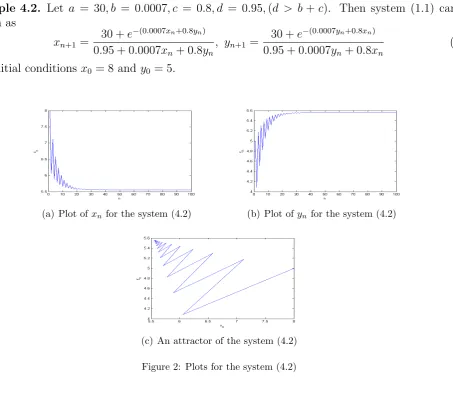
Example 4.2. Let a = 30, b = 0.0007, c = 0.8, d = 0.95,(d > b +c). Then system (1.1) can be written as

xn+1 =

30 +e−(0.0007xn+0.8yn)

0.95 + 0.0007xn+ 0.8yn

, yn+1 =

30 +e−(0.0007yn+0.8xn)

0.95 + 0.0007yn+ 0.8xn

(4.2)

(10)

In this case, the unique positive equilibrium point of the system (4.2) is given by

(¯x,y) = (5.557681533,¯ 5.557681533).

Moreover, in Figure 2, the plot of xn is shown in Figure 2 (a), the plot of yn is shown in Figure 2

(b), and an attractor of the system (4.2) is shown in Figure 2 (c).

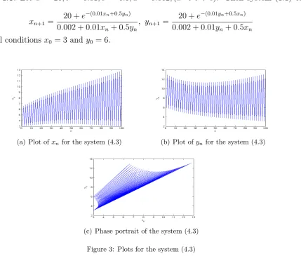
Example 4.3. Let a = 20, b = 0.01, c = 0.5, d = 0.002,(d < b+c). Then system (1.1) can be written as

xn+1 =

20 +e−(0.01xn+0.5yn)

0.002 + 0.01xn+ 0.5yn

, yn+1 =

20 +e−(0.01yn+0.5xn)

0.002 + 0.01yn+ 0.5xn

(4.3)

(c) Phase portrait of the system (4.3) Figure 3: Plots for the system (4.3)

In this case, the unique positive equilibrium point of the system (4.3) is unstable. Moreover, in Figure 3, the plot ofxnis shown in Figure 3 (a), the plot of yn is shown in Figure 3 (b), and a phase

portrait of the system (4.3) is shown in Figure 3 (c).

References

[1] R.P. Agarwal,Difference Equations and Inequalities, Second Ed. Dekker, New York, 2000.

[2] DˇZ. Burgi´c and Z. Nurkanovi´c, An example of globally asymptotically stable anti-monotonic system of rational difference equations in the plane, Sarajevo J. Math. 5 (2009) 235–245.

[3] E. El-Metwally, E.A. Grove, G. Ladas, R. Levins and M. Radin,On the difference equation,xn+1=α+βxn−1e−xn,

Nonlinear Anal. 47 (2001) 4623–4634.

[4] E.A. Grove and G. Ladas,Periodicities in Nonlinear Difference Equations, Chapman and Hall, CRC, 2005. [5] V.V. Khuong and M.N. Phong,On the system of two difference equations of exponential form, Int. J. Difference

Equ. 8 (2013) 215–223.

(11)

[7] Kulenovi´c, M. R. S. and G. Ladas,Dynamics of Second Order Rational Difference Equations with Open Problems and Conjectures, Chapman and Hall/ CRC, Boca Raton, London, 2001.

[8] M.R.S. Kulenovi´c and Z. Nurkanovi´c,The rate of convergence of solution of a three dimensional linear fractional systems of difference equations, Zbornik radova PMF Tuzla - Svezak Matematika. 2 (2005) 1–6.

[9] M.R.S. Kulenovi´c and M. Nurkanovi´c,Asymptotic behavior of a competitive system of linear fractional difference equations, Adv. Difference Equ. Art. ID 19756 (2006) 13pp.

[10] I. Ozturk, F. Bozkurt and S. Ozen, On the difference equation yn+1 = (α+βe−yn)/(γ+yn−1), Appl. Math.

Comput. 181 (2006) 1387–1393.

[11] G. Papaschinopoluos, M.A. Radin and C.J. Schinas,On a system of two difference equations of exponential form:

xn+1=a+bxn−1e−yn, yn+1=c+dyn−1e−xn, Math. Comput. Model. 54 (2011) 2969–12977.

[12] G. Papaschinopoluos, M.A. Radin and C.J. Schinas, Study of the asymptotic behavior of the solutions of three systems of difference equations of exponential form, Appl. Math. Comput. 218 (2012) 5310–5318.

[13] M.N. Phong,A note on a system of two nonlinear difference equations, Elect. J. Math. Anal. Appl. 3 (2015) 170 –179.

[14] M. Pituk,More on Poincare’s and Peron’s theorems for difference equations, J. Difference Equ. Appl. 8 (2002) 201–216.

[15] G. Stefanidou, G. Papaschinopoluos and C.J. Schinas,On a system of two exponential type difference equations, Com. Appl. Nonlinear Anal. 17 (2010) 1–13.

[16] S. Stevi´c,On the recursive sequencexn+1=

α+βxn−1

1+g(xn), Indian J. Pure Appl. Math. 33 (2002) 1767–1774.

[17] S. Stevi´c,On a discrete epidemic model, Discrete Dyn. Nat. Soc. Article ID 87519 (2007) 10 pages.