Applications of Graph Operations

Applications of graph operations

M.TAVAKOLI AND F.RAHBARNIA

Department of Mathematics, Ferdowsi University of Mashhad, P. O. Box 1159, Mashhad 91775, Iran

(ReceivedJanuary 5, 2013; Accepted February 22, 2013)

ABSTRACT

In this paper, some applications of our earlier results in working with chemical graphs are presented.

Keywords: Topological index, graph operation, hierarchical product, chemical graph.

1.

INTRODUCTION

Throughout this paper all graphs considered are finite, simple and connected. The distance

dG(u,v) between the vertices u and v of a graph G is equal to the length of a shortest path

that connects u and v. Suppose G is a graph with vertex and edge sets V = V(G) and E = E(G), respectively, and e = abE(G). The set of edges of G whose distance to the vertex u

is smaller than the distance to the vertex v is denoted by M_uG(e). Then the edge PI index of

G, PIe(G), is defined as PIe(G) =



 

   



 _

E(G) uv e

G v G

u (e) M (e)

M [1,2]. In a similar way,

(e)

N_aG is defined as the set of vertices closer to the vertex a than to the vertex b. In other words, N_aG(e)= {u V(G) | d(u, a) < d(u, b)}. The vertex PI index of G, PIv(G), is defined

as [|N_uG(e)| + |N_vG(e)|] over all edges of G [3,4]. The edges e = uv and f = xy of G are said to be equidistant if min{dG(u, x), dG(u, y)}=min{dG(v, x), dG(v, y)}. For e = uv G, the set



of equidistant vertices of e is denoted by N₀G(e) and the set of equidistant edges of e is denoted by M₀G(e). Thenthe above definitions are equivalent to

PIv(G) = |V(G)||E(G)| –



E(G) e

G 0 (e)

N ,

PIe(G) = |E(G)|2 –



E(G) e

G 0 (e)

M .

A graph G with a specified vertex subset U V(G) is denoted by G(U). Suppose G

and H are graphs and U  V(G). The generalized hierarchical product, denoted by

G(U)H, is the graph with vertex set V(G) V(H) and two vertices (g, h) and (g′, h′) are adjacent if and only if g = g′ U and hh′  E(H) or, gg′  E(G) and h = h′. This graph operation has been introduced by Barriére et al. [5,6] and it has some applications in computer science. To generalize this graph operation to n graphs, assume that Gi = (Vi , Ei)

is a graph with vertex set Vi , 1 ≤ i ≤ N, having a distinguished or root vertex 0. The

hierarchical product H = GN …G2G1 is the graph with vertices the Ntuples xN …

x3x2x1, xi Vi , and edges defined by the following adjacencies:

xN…x3x2x1

                    0. 1 N x 2 x 1 x ) N E(G N y N x 1 x 2 x 3 x N y 0, 2 x 1 x ) 3 E(G 3 y 3 x 1 x 2 x 3 y N x 0, 1 x ) 2 E(G 2 y 2 x 1 x 2 y 3 x N x ), 1 E(G 1 y 1 x 1 y 2 x 3 x N x ... and if ... : : : and if ... and if ... if ...

We encourage the reader to consult [7] for the mathematical properties of the hierarchical product of graphs.

2.

MAIN RESULTS

Let G = (V, E) be a graph and U  V. Following Pattabiraman and Paulraja [8], an u–v path through U in G(U) is an u–v path in G containing some vertex w  U (not necessarily distinct from the vertices u and v). Let dG(U)(u,v) denote the length of a shortest u –v path

through U in G. Notice that, if one of the vertices u and v belong to U, then dG(U)(u,v) =

dG(u,v). A vertex xV(G(U)) is said to be equidistant from e = uvE(G(U)) through U in

G(U), if dG(U)(u, x) = dG(U)(v, x). For an edge e = ab in G(U), let N₀G(U)(e) denote the set of

equidistant vertices of e through U in G(U) and N_aG(U)(e) denote the set of vertices closer to a than to b through U in G. Then PIv(G(U)) and PIe(G(U)) can be computed by the

PIv(G(U)) =



 

   



 _

E(G(U)) ab

e

G(U) b G(U)

a (e) N (e)

N

= |V(G(U))||E(G(U))| –



E(G(U)) e

G(U) 0 (e)

N .

The edges e = uv and f = xy of G(U) are said to be equidistant edges through U in

G(U) if

min{dG(U)(u, x), dG(U)(u, y)}= min{dG(U)(v, x), dG(U)(v, y)}.

Let M₀G(U)(e) denote the set of equidistant edges of e through U in G(U) and M_aG(U)(e) denote the set of edges closer to a than to b through U in G. Then PIe(G(U)) is computed as

follows:

PIv(G(U)) =



 

   



 _

E(G(U)) ab

e

G(U) b G(U)

a (e) M (e)

M

= |E(G(U))|2 –



E(G(U)) e

G(U) 0 (e)

M .

Theorem 1. [9]. Let G and H be two connected graphs and let U be a nonempty subset of

V(G). Then PIv(G(U)  H) =|V(H)| (|V(H)| – 1) PIv(G(U)) + |V(H)|PIv(G) +

|V(G)||U|PIv(H).

Theorem 2. [9]. Let G and H be two connected graphs and let U be a nonempty subset of

V(G). Then

PIe(G(U) H) = |V(H)|(|V(H)| – 1)PIe(G(U)) + |V(H)|PIe(G)

+ |V(H)||E(H)|

(

|U||E(G)| –



 

 

E(G(U)) g

g

G(U)

0 (gg) U

N

)

+ |E(G)||U|PIv(H) +|U|2PIe(H).

We are now ready to obtain the PI indices of some chemical graphs.

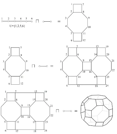
Example 3. Let H be the graph of truncated cuboctahedron (see Figure 1). Then H =

((P6(U1) P2)(U2) P2)(U3) P2, where U1 = {1, 2, 5, 6}, U2 = {7, 9, 10, 12} and U3 =

{1, 3, 4, 6, 19, 21, 22, 24}. One can see that PIe(P6(U1) P2) = 2  20 + 2  20 + 2 

(4  5) + 5  4  2 = 160. Also PIe((P6(U1) P2)(U2) P2) = 2  176 + 2  160 + 2  4 

14 + 14  4  2 = 896. Thus, by Theorem 1, we have

Figure 1. The Molecular Graph of Truncated Cuboctahedron.

Example 4. Octanitrocubane is the most powerful chemical explosive with formula

C8(NO2)8), part (a) of Fig. 2. Let H be the molecular graph of this molecule. Then obviously

H= P4(U)Q2, where U = {2, 3}. On the other hand, one can easily see that PIe(P4(U))=8

and PIe(P4) = 6 and so, by Theorem 1, we have

Figure 2. The Molecular Graph of Octanitrocubane.

Figure 3. The BridgeCycle Graph.

Example 5. Let

 

G_{i i}d_1 be a set of finite pairwise disjoint graphs with viV(Gi). The

bridgecycle graph BC(G1, G2, …, Gd) = BC(G1, G2, …, Gd; v1, v2, …, vd) of

 

G_{i i}d₁ with

respect to the vertices

 

v_i d_i1 is the graph obtained from the graphs G1, …, Gd by

connecting the vertices vi and vi+1 by an edge for all i = 1, 2, …, d –1 and connecting the

BC(G1, G2, … , Gd)  G(U) Cd, where |U|=|{r}|=1. On the other hand, It is not so

difficult to check that PIe(Cn)=

      n | 2 2) n(n n | 2 1) n(n

and PIv(Cn)=

     n | 2 n n | 2 1) n(n

2 . Therefore, if

2 | m, by Theorem 1, we have PIe(G(U)Cm) = m(m – 1)PIe(G(U)) + mPIe(G) +

m2(2|E(G)| – Nr(G)) + m(m – 2) and if 2 | m, then PIe(G(U)Cm) = m(m – 1)PIe(G(U)) +

mPIe(G) + m2(2|E(G)| – Nr(G)) – m|E(G)| + m(m – 1), where Nr(G)=|{uvE(G) |

dG(u,r)=dG(v,r)}|.

By replacing G with Pn (such that r is a pendant vertex of Pn) in the above relations,

we obtain PIe of Sunm, n–1, see [10], as follow:

PIe(Sunm, n–1)=

         m | 2 m mn n m m | 2 m 2mn n m 2 2 2 2 .

In what follows, let j f 1

i i 



and



j 0

i fi for each i, j {0, 1, 2, …}, that i – j

= 1. Furthermore, let f j f 0

i i j

i i 







for every i, j {0, 1, 2, …}, such that i – j > 1.

Also, for a sequence of graphs, G1, G2, …, Gn, we set 



_

j i

k k

j

i, V(G )

V and



   j l k i, k k l j

i, V(G )

V .

Theorem 6. [11]. Suppose G1, G2, …, Gn are connected rooted graphs with root vertices r1,

…, rn, respectively. Then

PIe(Gn …G2G1) = V PI (G ) V E(G )V PIv(Gi) -1 i 1 j 1 i 1, j j n 1 i n 1, i n 1 i i e n 1,

i _

      







       +





     n 1 i n 1 i j j n 1, i r

i) N )V ((V(G ) 1)

E(G ((

i

= E(G )V E(G ))) 1 j 1 k j 1 j 1, k k



     ,

where N_r



uv E(G_i)|d_G(u,r_i) d_G(v,r_i)



i i

i    .

Example 7. Let Γ be the graph of octanitrocubane, see part (b) of Figure 6. Then obviously

H= Q3 P2. On the other hand, one can easily see that PIe(Q3) = PIv(Q3) = 96 and PIe(P2)

REFERENCES

1. P. V. Khadikar, S. Karmarkar, A novel PI index and its applications to QSPR/QSAR studies, J. Chem. Inf. Comput. Sci.41 (2001) 934–949.

2. P.V. Khadikar, On a novel structural descriptor PI, Nat. Acad. Sci. Lett. 23 (2000) 113–118.

3. M. H. Khalifeh, H. YousefiAzari and A. R. Ashrafi, Vertex and edge PI indices of Cartesian product graphs, Discrete Appl. Math.156 (2008), 1780–1789.

4. M. H. Khalifeh, H. YousefiAzari, A. R. Ashrafi, A matrix method for computing Szeged and vertex PI indices of join and composition of graphs, Linear Algebra Appl.429 (2008) 2702–2709.

5. L. Barriére, F. Comellas, C. Daflo and M. A. Fiol, The hierarchical product of graphs, Discrete Appl. Math.157 (2009) 36–48.

6. L. Barriére, C. Dao, M. A. Fiol and M. Mitjana, The generalized hierarchical product of graphs, Discrete Math.309 (2009) 3871–3881.

7. M. Tavakoli, F. Rahbarnia and A. R. Ashrafi, Distribution of some graph invariants over hierarchical product of graphs, Appl. Math. Comput. 220 (2013) 405–413. 8. K. Pattabiraman, P. Paulraja, Vertex and edge PadmakarIvan indices of the

generalized hierarchical product of graphs. Discrete Appl. Math. 160 (2012) 1376– 1384.

9. M. Tavakoli, F. Rahbarnia, A. R. Ashrafi, Applications of Generalized Hierarchical Product of Graphs in Computing the Vertex and Edge PI Indices of Chemical Graphs, to appear in Ricerche di Matematica.

10.Y. N. Yeh and I. Gutman, On the sum of all distances in composite graphs, Discrete Math. 135 (1994) 359–365.