Integrating a 2D Hydraulic Model and GIS Algorithms into a Data Assimilation Framework for Real Time Flood Forecasting and Mapping

Integrating a 2D hydraulic model and GIS

algorithms into a data assimilation framework for

real time flood forecasting and mapping

Antonio Annis

_{, Noemi Gonzalez-Ramirez}

_{, Fernando Nardi}

_{, Fabio}

Castelli

1 _{WARREDOC, University for Foreigners of Perugia, Piazza Fortebraccio 4, 06123 Perugia, Italy}

2 _{DICEA, University of Florence, Via Santa Marta 3, 50139 Firenze, Italy}

3 _{Riada Engineering, Inc., P.O. Box 104, Nutrioso, AZ 85932, United States}

[email protected], [email protected], [email protected], [email protected]

Abstract

The intensification of flood-related damages and fatalities is challenging Early Warning Systems (EWS) to always better perform in predicting flood levels allowing decision makers to take the most effective decisions for mitigating the impact of extreme events. EWS require hydrologic and hydraulic modelling that are usually affected by uncertainties that can be extremely significant in data scarce regions. This work presents the implementation and application of a Data Assimilation (DA) framework, based on the Ensemble Kalman Filter, integrating the hydraulic model FLO-2D and geospatial algorithms for data post-processing and mapping. The hydraulic model is forced by both flow gages and simulated flow data produced by a simplified GIS-based hydrologic modelling for flood wave analysis tailored for small ungauged basins. The hydraulic code is adapted to assimilate different observation data types: flow measurements taken along the channel, water level observations captured within the floodplain, such as water signs on vegetation and buildings pictures by human sensors, and inundation extents obtained by processing satellite images. This DA framework required the development of significant novelties for incorporating the 2D hydraulic model and for integrating the different types of measurements considering the heterogeneous specifications and uncertainty of the various assimilated data types. Advanced GIS algorithms are implemented for improving the real time flood mapping taking advantage of the distributed output provided by the 2D inundation model. Results show improved model performances in terms of water level simulations and reduced uncertainties. The integrated hydraulic and geospatial modelling allows to empower the water levels correction on the flood extension prediction. Additionally, the capability of using the different available observations, from satellite images to crowdsourced data, is promising

Volume 3, 2018, Pages 36–44

for the development of a flexible and scalable flood EWS model overcoming the limitations of standard DA working generally with 1D hydraulic models and traditional sensors.

1

Introduction

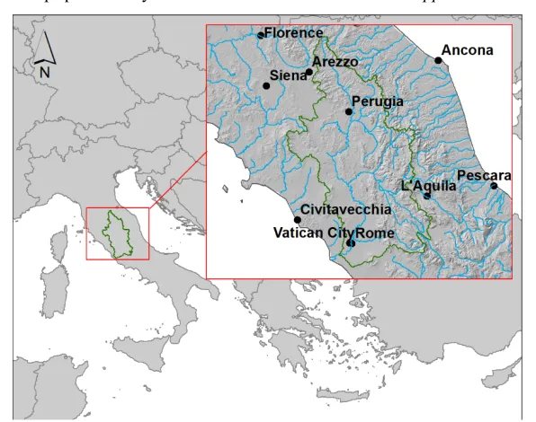
The increasing impact and occurrence of extreme events together with the demographic expansion in riverine areas are causing the dramatic surge of flood-related damages and fatalities (Jongman et al.2014) . Early Warning systems (EWS) are useful tools for predicting the flood levels allowing timely and efficient decision making to manage water disasters and mitigate economic losses and disruptions in urban areas (Plate, 2002). However, hydrologic observations are not sufficient for EWS and hydrologic and hydraulic models are required. The complexity of integration of hydro-modelling tools with heterogeneous observations challenge EWS to consider and manage the significant modelling uncertainties. Data Assimilation (DA) methodologies allow to reduce this uncertainty by efficiently incorporating different simulated and observed data while updating the states, inputs or parameters of the core flood modelling algorithm. Usually DA methodologies for flood modelling are quite computationally intense, so that simplified 1D hydraulic models and lumped hydrologic information are usually adopted for their simplicity and reduced computational burden. Nevertheless, 1D models are characterized by significant limitations in the reproduction of the distributed flood wave dynamics. Moreover, DA methodologies generally implement measurements taken from fluvial stage stages and more recently also considering data gathered from satellite sensors (Krzhizhanovskaya et al., 2011). In this work, we explore and test the performances of a novel DA framework integrating a Quasi-2D hydraulic model for flood risk modelling and mapping assimilating the different available measurements considering both traditional single water stages, inundation extents from satellite images as well as distributed or crowdsourced observations taken within the entire floodplain domain. The Tiber river basin is selected as case study considering the 120 km river reach that flows upstream of the city of Rome for its strategic importance in the flood risk mitigation of the historical urbanized area as well as for the availability of traditional and informal crowdsourced hydrologic information gathered in most recent flood events.

2

Material and methods

2.1

Available data

For the Tiber river case study (Figure 1), the following data were available:

• In situ surveyed cross sections provided by Autorità di Bacino distrettuale dell’Appennino

Centrale.

• Lidar (1 meter resolution) covering most of the floodplain area of the Tiber River provided

by the National Cartographic Portal (Portale Cartografico Nazionale or PCN) by the Italian

Ministry of Environment.

• DEM (5 meters resolution) from Regione Lazio and Tinitaly 10 meter resolution from Istituto

Nazionale di Geofisica e Vulcanologia (INGV) (Tarquini et al., 2007).

• Rain and stage gages time series for historical flood events provided by Regione Lazio and

• Land use map from Istituto Superiore per la Protezione e la Ricerca Ambientale (ISPRA) and

soil types maps provided by Autorità di Bacino distrettuale dell’Appennino Centrale.

2.2

Hydrologic modelling

The hydrologic input for the hydraulic model is given by the available stage gages for the main river channel. Ungauged tributary basins are simulated using a parsimonious hydrological model following (Grimaldi et al., 2012; Nardi et al., 2018) and implemented in python environment. The rainfall-runoff model is based on the DEM-based geomorphic characterization of runoff production dynamics tailored for scarcely monitored river basins with specific regard to the WFIUH method (Mesa, & Mifflin, 1986) namely the instantaneous unit hydrograph (IUH) concept, estimated using the width function (WF). Specifically, for each time step, the IUH is given by the percentage of basin contributing to the basin outlet, starting from the distribution of the cell by cell flow velocities, determined considering the local slopes and the land uses, applying the NRCS method (NRCS, 1997)

2.3

Hydraulic modelling

The computational domain of the hydraulic model is identified using the DEM based hydro-geomorphic floodplain zoning algorithm developed starting from Nardi et al., (2006). The hydraulic model, FLO-2D PRO (O'brien, 1993) is selected for the ability to route flood hydrographs along channels (1D model) or over unconfined surfaces (2D model) also simulating the channel-floodplain exchange using the continuity equation and the dynamic wave approximation to the momentum equation. The model has been calibrated considering four stage gages along the Tiber river and validated for three flood events in 2005, 2010 and 2012. The core Quasi-2D hydraulic modelling component is adapted for its implementation within the DA framework in order to gather and process input data

dynamically, as hot starts, and automatically produce corrected flood wave routing results for EWS applications.

2.4

Data Assimilation model

FLO-2D is used as forecast model for the implementation of the DA method. Specifically, the Ensemble Kalman Filter (EnkF) method (Evensen , 2003) is applied.

The EnKF model is a sequential DA method that estimates the model state based on the observations at each time step they are available. The method is based on ensemble generations with Montecarlo simulations: the forecast (a priori) state error covariance matrix is approximated propagating the

ensemble of the model states 𝑥" using a forecast model and adding a random noise considering the

uncertainties of the model error.

The size of the ensemble is chosen adopting the methodology proposed by (Anderson, 2001). Following this approach, the ideal spread of the ensemble is reached with an ensemble size so that the Normalized RMSE Ratio (NRR) is close to 1 (See Anderson, 2001 for further details).

2.4.1.

Model error

The model error 𝑤" is estimated considering the uncertainties related by the input forcing and the

model parameters.

The input inflow 𝑄%

",'for the i-element of the ensemble at time t given by the stage gages and the

hydrologic model is expressed as suggested by Weerts & El Serafy (2006):

𝑄%

",' = 𝑄%"+ 𝑁(0, 𝑅") (1)

Where 𝑄%

" is the streamflow observation at time t, 𝑁(0, 𝑅") is a noise term normally distributed

with zero mean and a given variance (𝑅")at time t, expressed as:

𝑅_𝐼,𝑡 =

1𝛼

𝑡

5

Where α is the coefficient of variation related to the uncertainty of the input. In case of flow retrieved

from the rating curve tables related to the stage gages, α has been imposed equal to 0.12. For the

hydrologic model, the validation analysis suggested to impose α =0.3.

The uncertainty related to the model parameters is considered as follows:

𝑝𝑠_𝑖 = 𝑝𝑠+ 𝑈

(

)

Where 𝑝%

' is the perturbed model parameter for the i-element of the ensemble, 𝑝% is the model

parameter and 𝜀= is the fractional parameter error. In this case, the channel roughness has been chosen

as the perturbed parameter, with 𝑝%_{= 0.04 and 𝜀}

== 0.25.

2.4.2.

Implementation in 2D hydraulic modelling

The state variable 𝑥" is considered as the water depth in a specific point of the computational

crowdsourced information, namely a photo from which gathering the water depth or a description of the depth from a user, the state variable can be located in the channel, but more likely in the floodplain, where people usually could come across a flood event. The forecast model is the hydraulic model

engine, whose forcing term 𝐼" is the ensemble of the flow hydrographs and the parameters θ are mainly

the channel and floodplain roughness.

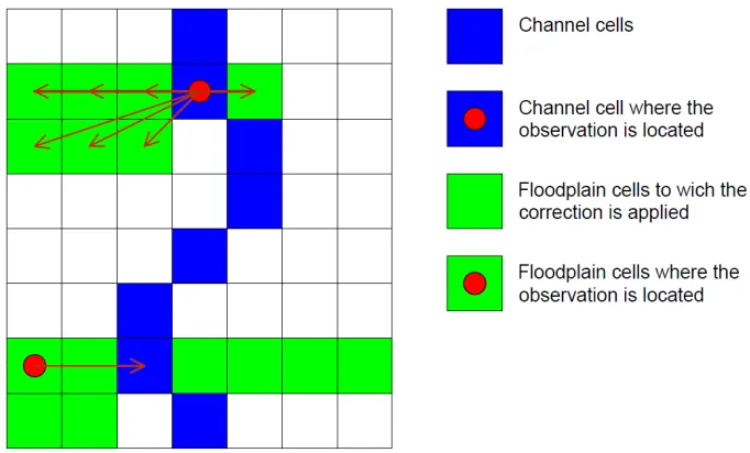
To assimilate stage gage measurements, the correction of the water depth is applied to the channel cell and to closest floodplain cells (Figure 2). The correction is also propagated upstream and downstream with a similar approach to Madsen & Skotner (2005) adopting a gain function that assigns a percentage of the whole correction calculated by the EnKF proportional to the inverse of distance between the channel cell where the correction is applied and the channel cell where the observation is available.

Furthermore, in order to simultaneously assimilate more than one stage gage observation, the portions of the channel (and its hydraulically connected floodplain) that is between two different stage observations, is updated considering both these observations using as weight the inverse of the distance of its connected channel cell from each stage gage cell.

Each time step when observation measurements are available, the hydraulic simulation is stopped and the water levels and volume conservation outputs are saved in binary files. Then the EnKF is applied and the water depth corrections are inserted in the binary files.

When the gain function is propagated upstream and the water level correction is positive, a counterslope of the water levels could occur, bringing the model to numerical instability. In order to avoid this, a further condition has been imposed: the absolute water level in the cell of the channel

𝐻D_(𝑥

') cannot be lower than the following downstream channel 𝐻D(𝑥')cell, but, at least, should be the

same.

The assimilation of flow depths derived from a satellite image can be summarised in the following steps:

• Flood detection from satellite image. The Water index introduced by (Fisher et al., 2016) has been adopted for detecting the water extension of the November 2012 flood.

• Comparison of the flood extent detected from the satellite image with the ensemble of flood

extents given by the hydraulic model. This procedure requires refining the resolution of the water surface elevation layer provided by the hydraulic model using a geostatistical technique involving the use of a high resolution DEM.

• Derivation of the water elevation profile along the channel from the satellite image starting

from the ensemble of the water elevation profiles of the hydraulic model.

In case of VGI observation in a floodplain cell or group of cells, the procedure identifies all closest channel cells related to the floodplain cells affected by observations. Than the correction is done to all the floodplain cells whose closest channel cells are the ones previously identified.

The water depth updating given by the DA procedure is propagated downstream and upstream using the gain function introduced by Madsen & Skotner (2005). In case of simultaneous assimilation of different VGI data, the gain function can be applied assigning a weight to the water level correction in a cell proportional to the inverse of the distance between the cell and each observation.

2.4.3.

Implementation in 2D hydraulic modelling

The perturbation 𝑣" to be assigned to the observation ensemble is strongly dependent on the nature

of the observation. In case of observations gathered from stage gages, the water depth for the i-element

of the ensemble at time t is given by:

𝑊𝐷H

I"I,",' = 𝑊𝐷I"I,""JKL+ 𝑁10, 𝑅I"I,'5 (4)

Where 𝑊𝐷I"I,""JKL is the observed water level by the static sensor (StS) at time t, 𝑁10, 𝑅I"I,',"5 is a

noise term normally distributed with zero mean and a given variance (𝑅I"I,',") at time t expressed as:

𝑅I"I,'," = 1𝛼I"I,'∙ 𝑊𝐷I"I,""JKL5 (5)

𝛼I"I,' is the coefficient of variation related to the uncertainty in the water level measurement,

assumed equal to 0.02.

The procedure for extracting the hydraulic profile from the satellite image is affected by a series of errors that have to be taken in to account when applied in a DA framework and here listed:

• Error in the water detection from satellite imagery (errOP): this error is due to 1) the water

detection technique 𝑒𝑟𝑟ST,IU that could overestimate and underestimate the water

extension; 2) the resolution 𝑒𝑟𝑟JL%,IU of the satellite image.

• Error of the water surface extraction from the WSE of the hydraulic model (errVW):This is

due to the vertical error of the DEM with which the interpolated water surface elevation is intersected.

• Error of the profile derivation from the ensemble of the hydraulic models (errXV).

• The observation errors related to VGI are given by the composition of three different

factors:

• Timing error: this can be the lag time between the information acquisition and the posting time or the error of the time directly indicated by the user during the content generation.

• Water depth estimation error, usually deduced by a subjective perspective without the

verification of an instrumental measure

3

Results

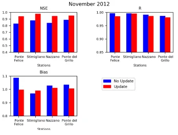
The November 2012 flood event is selected as test case. The case study is characterized by the assimilation of single (Static Sensors or StS; Crowdsourced data also known as Volunteered Geographic Information or VGI) and distributed measurements (water extension from Satellite Image or SI). Figure 3 shows performance indexes (Nash-Sutcliffe Efficiency-NSE, Pearson correlation – R, and Bias expressed as the ration between the sum of the simulated and the observed water levels) of the simulations implementing the proposed DA as respect to no-updated simulations derived using only the flood wave propagation model.

The assimilation of the StS is performed considering the first 50 hours hypothesizing a failure of the monitoring equipment. This worst case scenario is developed in order to test the effect of assimilating intermittent measurements that generally characterized SI and the VGI data of real events. Performances of the simulations, calculated considering the stage measurements as true observations, generally improve in case of updated simulations. However, the R coefficient results slightly lower in

case of DA application, because the intermittent observations assimilated by the model caused local increases of the mean water levels, modifying the natural curvature of the water levels time series.

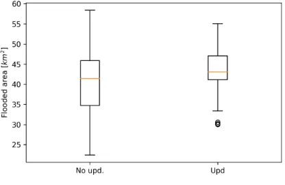
The assimilation of each measurement generates a narrowing of the ensemble spread that persists for 8 hours after the correction. The 2D simulation allows to calculate also the potential reduction of the flood extension uncertainty along the floodplain domain as shown in Figure 4.

4

Conclusions

The presented Data Assimilation framework includes the use of a Quasi-2D hydraulic model for improving the flood modelling and mapping for a fully dynamic and spatially distributed representation of floodplain inundation processes. The use of 2D models seems a promising way for improving the performances and mitigating the uncertainties of EWS for flood risk management consider that standard DA flood models currently rely on simplified 1D models,. Nevertheless, recent researchers usually consider only measurements from StS neglecting the availability and usefulness novel observation data such as water extensions taken from SI and Crowdsourced data (VGI). This approach tries to overcome these limitations incorporating into the DA any available measurement from both traditional and informal human-sensed information. Results confirm the potential capacity of the presented DA framework in improving EWS performances with specific regard to the improvements in representing the distribution of water levels and the reduced uncertainties in the simulation of the inundation extent.

References

Jongman, B., Hochrainer-Stigler, S., Feyen, L., Aerts, J. C., Mechler, R., Botzen, W. J., Bouwer, L. M., Pflug, G., Rojas, R.,Ward, P. J. (2014). Increasing stress on disaster-risk finance due to large floods. Nature Climate Change, 4(4), 264.

Plate, E. J. (2002). Flood risk and flood management. Journal of Hydrology, 267(1-2), 2-11.

Krzhizhanovskaya, V. V., Shirshov, G. S., Melnikova, N. B., Belleman, R. G., Rusadi, F. I., Broekhuijsen, B. J., …, Meijer, R. (2011). Flood early warning system: design, implementation and computational modules. Procedia Computer Science, 4, 106-115.

Tarquini, S., Isola, I., Favalli, M., Mazzarini, F., Bisson, M., Pareschi, M. T., & Boschi, E. (2007). TINITALY/01: a new triangular irregular network of Italy. Annals of Geophysics.

Grimaldi, S., Petroselli, A., & Nardi, F. (2012). A parsimonious geomorphological unit hydrograph for rainfall–runoff modelling in small ungauged basins. Hydrological Sciences Journal, 57(1), , 73-83. Nardi, F., Annis, A., & Biscarini, C. (2018). On the impact of urbanization on flood hydrology of small ungauged basins: the case study of the Tiber river tributary network within the city of Rome. Journal of Flood Risk Management, 11(S2), pp. S594-S603.

Mesa, O. J., & Mifflin, E. R. (1986). On the relative role of hillslope and network geometry in hydrologic response. In: V.K. Gupta, I. Rodriguez-Iturbe and E. F. Wood, Scale problems in hydrology, , 1–17. Dordrecht: D.Reidel.

NRCS (Natural Resources Conservation Service). (1997). Ponds-Planning, design, construction. Washington, DC: US Natural Resources Conservation Service, Agriculture Handbook no. 590 Nardi, F., Vivoni, E., & Grimaldi, S. (2006). Investigating a floodplain scaling relation using a

hydrogeomorphic delineation method. Water Resources Research, , 42 (9), 15 pp.

O'brien, J. S. (1992). Two-dimensional water flood and mudflow simulation. Journal of hydraulic engineering, 119(2), 244-261.

Evensen, G. (2003). The ensemble Kalman filter: Theoretical formulation and practical implementation. Ocean dynamics, 3(4), 343-367.

Anderson, J. L. (2001). An ensemble adjustment Kalman filter for data assimilation. Monthly weather review, 129(12), 2884-2903.

Weerts, A. H., & El Serafy, G. Y. (2006). Particle filtering and ensemble Kalman filtering for state

updating with hydrological conceptual rainfall-runoff models. . Water Resources Research, 42(9).

Madsen, H., & Skotner, C. (2005). Adaptive state updating in real-time river flow forecasting—A combined filtering and error forecasting procedure. Journal of Hydrology, 308(1), 302-312. Fisher, A., Flood, N., & Danaher, T. (2016). Comparing Landsat water index methods for automated

water classification in eastern Australia. Remote Sensing of Environment, 175, 167-182.