18
Developing Adaptive Differential Evolution as a New Evolutionary
Algorithm, Application in Optimization of Chemical Processes
B. Vaferi, A. Jahanmiri∗
Chemical and Petroleum Engineering School, Mollasadra Ave., Shiraz University, Shiraz, Iran
Abstract
Differential Evolution algorithm (DE), one of the evolutionary algorithms, is a new optimization technique capable of handling non-differentiable, non-linear and multimodal objective functions. DE needs a large run time for optimizing the complex objective function. Thus, an attempt to speed up DE is necessary. This paper introduces a modification on original DE that enhances the convergence rate by reducing vector dispersal at any iteration. Our Adaptive Differential Evolution algorithm (ADE) utilizes variable scaling parameter (F) against constant scaling parameter in original DE at any iteration. The proposed ADE is applied to optimize three non-linear chemical engineering problems. The obtained results have been compared with those results obtained using DE. The considered comparison criteria are the vectors dispersal, convergence history (run time and number of iterations that led to reach to global optimum)and error in any iteration. As compared to DE, ADE is found to perform better in locating the global optimal solution, reduces the memory and computational efforts by reducing the number of iterations required to reach the global optimal solution for all the considered problems.
Keywords: Global Optimization, Evolutionary Algorithm, Differential Evolution, Adaptive Differential Evolution, Variable Scaling Parameter
∗ Corresponding author: [email protected]
1- Introduction
Many engineering optimization problems have multiple optimal solutions, among them one or more may be the absolute optimum solutions. These absolute maximum or minimum solutions are known as global optimal solutions and the rest are known as local optimal solutions [1]. The reason for the popularity of global optimal solutions is that they can determine the absolute optimum
Iranian Journal of Chemical Engineering, Vol.8, No. 1 19
traditional methods [2]. In the recent past year, non-traditional search and optimization techniques based on natural phenomenon, such as genetic algorithms [3], evolution strategies [4], simulated annealing [5], bird migration [6] and Differential Evolution [7], have been applied to solve the problems. Some of advantages of Differential Evolution are as follows:
1- They can be applied to the non-continuous and/or non-differentiable objective functions.
2- They are not sensitive to the initial point. 3- They usually do not get trapped into local
optimal solutions.
2- Differential evolution
DE, invented as a result of Price and Storn's study in 1995, is a simple powerful population based technique for finding the global optimal solution of non-differentiable, nonlinear and multi-modal optimization problems [7]. This technique combines simple arithmetic operators with the classical events of mutation, crossover and selection to evolve from an accidentally generated initial population (consisting of NP member vectors xi,G(i=1,2,...,NP for each
generation) to the final individual solution. Mutation and crossover are used to generate new vectors (trial vectors), and selection then determines which of the vectors will go on into the next generation. Specific design of generating trial parameter vectors as explained earlier is a key idea behind the DE. According to Storn and Price's work, DE’s basic strategy can be described as follows:
3- Mutation
A mutant vector is produced for each target
vector xi,G, (i =1, 2, ..., NP), according to Eq.
(1):
(
r G r G)
G r G
i x F x x
v, +1= 1, + * 2, − 3,
1
r ≠ r2 ≠ r3 ≠I (1)
With accidentally selected integer indexes r1, r2, r3 that belong to {1, 2, ..., NP}. Note that indexes must be dissimilar from each other and from the running index. F has a value between [0, 2] which controls the strengthening of the differential variation (xr2,G−xr3,G).
4- Crossover
In order to enhance the diversity of the perturbed parameter vectors, crossover is added. The target vector is mixed with the mutated vector, using the Eq. (2), to yield the trial vector.
D j
otherwise x
i rnbr j or CR j b rand if v
u
G ji
G ji G ji
..., , 2 , 1
) ( )
) ( (
, 1 , 1 ,
= ⎪⎩
⎪ ⎨
⎧ ≤ =
= +
+
(2)
Where randb(j) is the jth evaluation of an identical random number producer between [0, 1]. CR is the crossover constant between [0, 1] which has to be entered by the user. rnbr(i) is a randomly selected index from 1, 2, . . . , D which guarantees that the trial vector gets at least one parameter from the target vector. Otherwise, no new parent vector would be formed and the population would not change.
5- Selection
20 Iranian Journal of Chemical Engineering, Vol. 8, No. 1
vector should become a member of the next generation, the trial vector is compared to the target vector by using the specified criterion. Suppose that the objective function should be minimized. According to the Eq. (3):
⎪⎩ ⎪ ⎨
⎧ ≤
= + +
+
otherwise x
x f u
f if u
x
G i
G i G
i G
i G
i
,
, 1
, 1
, 1 ,
)) ( ) (
(
(3)
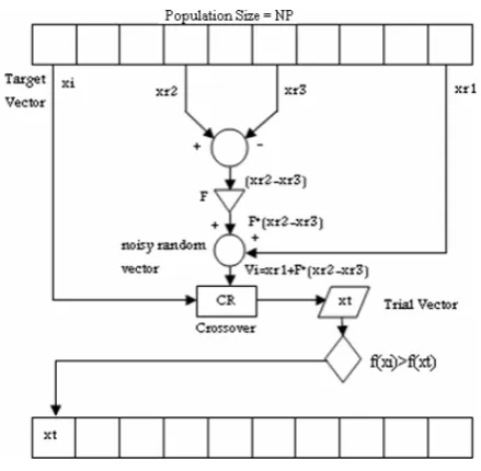
If the trial vector yields a better value of the objective function than the target vector, then the target vector is replaced with the trial vector. Otherwise, the old value of target vector is retained. As a result, all the individuals of the next generation are as good as or better than their counterparts in the present generation. In should be mentioned that the trial vector is only compared to one individual vector, not to all the individual vectors in the present population. The schematic figure of the original DE algorithm is shown in Fig. 1.
Figure 1. Schematic diagram of original DE
6- Constraint handling
Many engineering optimization problems have a constraint. The complexity of utilizing Evolutionary Algorithms in the constrained optimization problem is that the evolutionary operators utilized to manipulate the individuals of the population often generate solutions which are unfeasible. The constraint handling in the present study is performed based on the penalty function method. This technique transforms the constrained problem into an unconstrained problem by penalizing unfeasible solutions according to Eqs. (4, 5).
Minimize f (X)
subject to g(X) Minimize: P (f ,g, h, r) h(X)
⎫ ⎪ ⇒ ⎬ ⎪ ⎭
(4)
{
}
[
]
21 1
2
2( , ) ( ) (
∑
( )∑
max 0, ( )= =
+ +
= r
j
j m
j
j g
h r f r
p x x x x
(5)
7- Improvement on differential evolution The principle of ADE is the same as the original DE. The major difference between ADE and DE is that our algorithm uses variable scaling parameter against constant scaling parameter in the original DE at any iteration. F controls the amplification of the differential variation
(
Xr2,G−Xr3,G)
in the mutation step based on Eq. (1). It can be said that variable F can reduce solution vectors dispersal in any iteration and results in faster convergence.Iranian Journal of Chemical Engineering, Vol.8, No. 1 21
results suggest that square function has the best performance to reduce vector dispersal in any iteration, and therefore can result in faster convergence. Scaling parameter is updated by the square function according to Eq. (6), as and when an iteration progresses. B is a parameter that reduces with the progress of the iteration and results in reducing the value of F. That parameter is defined in Eq. (7).
(
)
21 i 1 i
i F B
F + = × − (6)
i i
F B
Maximum number of iterations
= (7)
It has been shown that F0=0.8 is the best
value of scaling parameter. Thus, in the present study, F0= 0.8 is used as an initial
value.
8- Examination of vector dispersal of ADE and DE
The investigation of vector dispersal of the proposed ADE and the original DE has been carried out by finding an optimal solution of two dimensions optimization problem. Based on Eq. (8), the objective function should be minimized subject to equal and non equal constraints that are defined by Eq. (9).
2 2
1 2
Minimize: f (X) (x 1)= − +x (8)
2 2
1 2 1 2
Subject to: h(X) x= +x + +x x =0
2
1 2
g(X) = − +x x ≥0 (9)
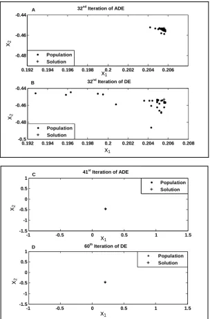
In the Fig. 2(A) and 2(B), the vector dispersal of ADE and DE with 30 members has been shown in the 32nd iteration. The Fig. 2(A) and 2(B) clearly show that the vector dispersal of ADE is less than that obtained by
DE. As can be seen from Fig. 2(C) and 2(D), the proposed ADE located the global optimal solution after 41 iterations, while the original DE reached the global optimal solution after 60 iterations. In Fig. 2(C) and 2(D), all of the members of ADE and DE coincide with the optimal solution located in X = [0.2056, -0.4534]. The actual global optimal solution is shown by asterisk in Fig. (2).
The variable scaling parameter that is utilized in the ADE algorithm, results in reducing vector dispersal in any iteration and finding a global optimal solution in a lower number of iterations. In fact, the lower vector dispersal led to a reduction of the required time to reach a global optimal solution. These issues are investigated in more detail through three non linear chemical engineering optimization problems.
9- Optimization of non-linear chemical processes
The proposed ADE is applied to optimize three non-linear chemical process problems. The performance of ADE and DE is compared. The comparison is made by considering the convergence history (run time and the number of runs converged to global optimal solution) and errors in any iteration.
9.1- Minimizing company's total costs
A company has two alkylate units, A1 and A2, from these, a product is sent to customers, C1, C2, and C3. The transportation expenses are given in Table (1).
22 Iranian Journal of Chemical Engineering, Vol. 8, No. 1 0.192 0.194 0.196 0.198 0.2 0.202 0.204 0.206
-0.48 -0.46 -0.44
32 th Iteration of ADE
x2
x1
0.192 0.194 0.196 0.198 0.2 0.202 0.204 0.206 0.208 -0.5
-0.48 -0.46 -0.44
x1
x2
32 th Iteration of DE Population
Solution
Population Solution A
B
-1 -0.5 0 0.5 1 1.5
-1.5 -1 -0.5 0 0.5 1
60th Iteration of DE
x1
x2
Population Solution
-1 -0.5 0 0.5 1 1.5
-1.5 -1 -0.5 0 0.5 1
x1
x2
41th Iteration of ADE
Population Solution C
D
Figure 2. Schematic of vector dispersal in 32nd (A), (B) and final iteration (C), (D) of ADE and original DE.
Table 1. The transportation costs between plants and customers
Refinery A1 A1 A1 A2 A2 A2
Customer C1 C2 C3 C1 C2 C3
Cost ($/ton) 25 60 75 20 50 85
Table 2. The maximum refinery production rates and minimum customer demand rates
Customer or production A1 A2 C1 C2 C3
Rate (ton/day) 1.6 0.8 0.9 0.7 0.3
32nd Iteration of ADE
32nd Iteration of DE
41st
Iteration of ADE
60th
Iteration of DE
x2
x2
x2
x2
x1
x1
x1
Iranian Journal of Chemical Engineering, Vol.8, No. 1 23
For production levels less than 0.5(ton/day),
the cost of production for A1 is
30(dollars/ton), while it is 40(dollars/ton) for production levels greater than 0.5 (ton/day), A2's production cost is uniform at 35(dollars/ton). The objective is finding the optimum distribution policy to minimize the company's total costs [1]. The optimal and the optimal variable values are: f =151.4934,
X = [0.7999, 0.0000, 0.2999, 0.1001, 0.7000, 0.0000].
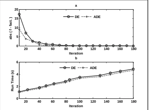
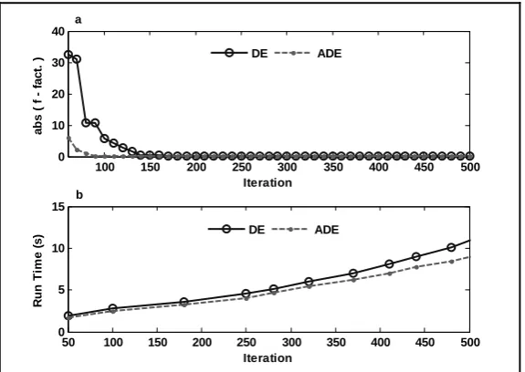
Errors and required CPU time for reaching an optimal solution at any iteration, by using DE and ADE algorithm are shown in Fig. 3(a) and 3(b), respectively. It should be mentioned that, in Fig 3(a), error is defined as an absolute (f-fact.) where f and fact are
optimal solution in any iteration (get via optimization algorithm) and actual optimal solution (get from literature), respectively. It can be seen from Fig. 3(a), that the errors that have been obtained via ADE were smaller than those that have been gotten from DE at any iteration. Error has reached zero by ADE after 100 iterations, while the error of the DE algorithm at the 180th iteration is
equal to zero. It can be seen from Fig. 3(b) that ADE also reduces the required CPU and run time to reach a global optimal solution. The differences between the computational efforts of two algorithms have increased as the iteration progresses. These statuses have been accessed for all the considered problems. The values of the objective function that have been calculated by ADE and DE are shown in Table (3).
9.2- Optimal operation of alkylation unit
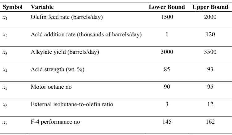
Alkylation is a common unit in the petroleum industry. As shown in Fig. 4, a butane feed, a pure isobutane recycle and a 100% isobutane make-up stream are fed into a reactor, together with an acid catalyst. The reactor product is then fed into a fractionator where the isobutane and the alkylate product are separated. The spent acid is also removed from the bottom of the reactor. The variables are defined as shown in Table (4) along with the upper and lower bounds on each variable. The bounds represent physical, economic and performance constraints [8].
20 40 60 80 100 120 140 160 180
0 5 10 15 20
a
Iteration
a
b
s ( f
- fa
ct.
)
20 40 60 80 100 120 140 160 180
0 2 4 6
b
Iteration
Ru
n
T
im
e
(
s
)
DE ADE
DE ADE
24 Iranian Journal of Chemical Engineering, Vol. 8, No. 1
Table 3. Objective function value of ADE and DE
Iteration Objective function value of DE Objective function value of ADE
10 168.856778 160.502563
30 154.000476 154.081014
50 152.371523 151.673524
70 151.917102 151.535829
90 151.547618 151.493786
100 151.511981 151.493356
130 151.496358 151.493356
180 151.493357 151.493356
180 151.493356 151.493356
Figure 4. alkylation process flow sheet
Table 4. variables and their bounds
Symbol Variable Lower Bound Upper Bound
x1 Olefin feed rate (barrels/day) 1500 2000
x2 Acid addition rate (thousands of barrels/day) 1 120
x3 Alkylate yield (barrels/day) 3000 3500
x4 Acid strength (wt. %) 85 93
x5 Motor octane no 90 95
x6 External isobutane-to-olefin ratio 3 12
Iranian Journal of Chemical Engineering, Vol.8, No. 1 25
In the present study, the problem formulation is the same as that of Maranas and Floudas (1997) and Adjiman et al. (1998). The
objective function and related constraints are shown through Eq. (10) and (11), respectively: 5 3 2 3 6 1
1 0.035 4.0565 10 0.063
715 .
1 x xx x x x x
profit
Max = + + + − (10)
to Subject 0 1175625 . 0 88392857 . 0 0059553571 .
0 x62x1+ x3− x6x1−x1≤
0 0066033 . 0 1303533 . 0 1088 .
1 x1+ x1x6− x1x62−x3≤
0 10000 20592 . 191 596669 . 56 39878 . 172 66173269 .
6 x62+ x5− x4− x6− ≤
0 85075 . 56 03762 . 0 32175 . 0 08702 .
1 x6+ x4− x62−x5+ ≤
0 125634 . 25 3121 . 2462 006198 .
0 x7x4x3+ x2− x2x4−x3x ≤ 0 489510
5000 18996
.
161 x3x4+ x2x4 − x2 −x3x4x7 ≤
0 333333 . 44 33 .
0 x7 −x5+ ≤
0 0 . 1 00759 . 0 022556 .
0 x5− x7− ≤
0 0 . 1 0005 . 0 00061 .
0 x3 − x1− ≤
0 819672 . 0 819672 .
0 x1−x3+ ≤
0 250
24500x2− x2x4−x3x4 ≤
0 100000 2244898 . 1 4082 .
1020 x4x2+ x3x4− x2 ≤
0 100000 625 . 7 25 . 6 25 .
6 x1x6+ x1− x3− ≤
0 0 . 1 22 .
1 x3−x6x1−x1+ ≤
(11)
The maximum profit as reported in [8] is,
177277 (dollars/day) and the optimal variable
values are:
x1 = 1698.18, x2 = 53.66, x3 = 30313, x4 = 90.11, x5 = 95, x6 = 10.50, x7 = 153.33.
In this problem the error is defined the same as the previous one. The obtained information has been plotted in Fig. 5(a) and 5(b). In the current problem, ADE has shown a smaller error than DE in any iteration too. ADE and DE algorithms have reached real optimal solution (very small value for error) after 125 and 230 iterations, respectively. In other words, fewer iterations are required for reaching a global optimal solution using
ADE compared to the original DE. Required CPU time for reaching an optimal solution in any iteration is shown in Fig. 5(b). The required computational times of the original DE are higher than those ADE needed, and the differences become larger as the iterations progress.
9.3- Heat exchanger network design
26 Iranian Journal of Chemical Engineering, Vol. 8, No. 1
100 150 200 250 300 350 400 450 500 0
10 20 30 40
Iteration
ab
s (
f
- fact.
)
50 100 150 200 250 300 350 400 450 500 0
5 10 15
Iteration
R
u
n Ti
m
e
(
s
) DE ADE
DE ADE
b a
Figure 5. Error (a) and Run Time (b) vs. Iteration for DE and Proposed ADE
Figure 6. Heat exchanger network design
The problem formulation has been taken from Floudas and Pardalos (1990). Objective
function and related constraints are shown through Eq. (12) and (13):
3 2
1 x x
x f
Minimize = + + (12)
to subject
0 333 . 83333 332
. 833 ) 400 (
100x1−x1 −x4 + x4+ ≤ 0 1250 1250
) 400
( 5 4 4 5
2 4
2x −x −x +x − x + x ≤
x
0 1250000 2500
) 100
( 5 5
3 5
3x −x +x − x + ≤
x
1000 ,
10 , 10000 ,
1000 , 10000
100≤x1 ≤ ≤x2 x3 ≤ ≤x4 x5 ≤
(13)
The global optimal as reported in [9] is: (x1,
x2, x3, x4, x5, x6, x7, x8; f) = (579.19, 1360.13, 5109.92, 182.01, 295.6, 217.9, 286.4, 395.6, 7049.25).
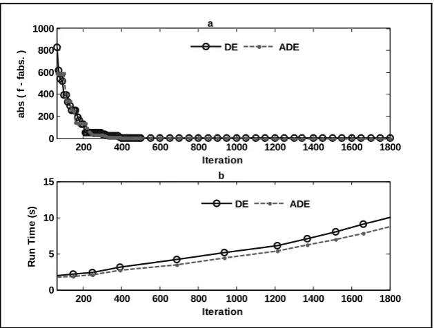
As were seen in the previous problems, ADE shows a smaller error and the required
Iranian Journal of Chemical Engineering, Vol.8, No. 1 27
shown in Fig. 7(a), at the 1100th and the 1900th iterations, the value of error reached zero (real optimal solution), by ADE and DE, respectively. It can be seen from Fig. 7(b),
that ADE also requires a smaller memory and computational efforts to reach a global optimal solution.
200 400 600 800 1000 1200 1400 1600 1800 0
5 10 15
Iteration
Ru
n
T
im
e
(s
) DE ADE
200 400 600 800 1000 1200 1400 1600 1800 0
200 400 600 800 1000
Iteration
a
b
s
( f
fa
b
s
. ) DE ADE
b a
Figure 7. Error (a) and Run Time (b) vs. Iteration for DE and ADE
10- Conclusions
Utilizing variable scaling parameter in the mutation step is the main difference between the proposed ADE and the original DE. Variable scaling parameter results in reducing vector dispersal, reducing error and run time at any iteration. The proposed ADE and original DE have been applied to optimize three non-linear chemical engineering problems. The results obtained from ADE have been compared with those using DE, by considering the convergence history and error in any iteration. As compared to DE, ADE is found to perform better in locating the global optimal solution for all the considered problems. ADE also reduces the memory and computational
efforts by reducing the number of iterations to reach a global optimal solution.
11- Nomenclature
ADE Adaptive Differential Evolution
CR crossover constant
DE Differential Evolution
f objective function
F scaling parameter
NP population size
Run-time time taken by CPU per execution uji,G Trial vector
vi, G
noisy random vector, ith dimension in (G+1)th generation
xi,G Target vector
28 Iranian Journal of Chemical Engineering, Vol. 8, No. 1 References
[1] Edgar, T. F., and Himmelblau, D. M., Optimization of chemical processes, 2nd ed., McGraw-Hill, Inc., Singapore, p. 118 and 202 and 261 (2001).
[2] Onwubolu, G. C., and Babu, B.V., New optimization techniques in Engineering, 1st ed., Springer, Heidelberg, Germany, p. 54-60 (2004).
[3] Holland, J. H., Adaptation in natural and artificial systems, Michigan, 5th ed., the University of Michigan Press, Michigan, USA, p. 32-36 (1998).
[4] Schwefel, H. P., Numerical optimization of computer models. New York, 1st., ed., John Wiley & Sons, p. 256 (1981).
[5]Kirkpatrick, S., Gelatt, C. D., and Vechhi, M. P., "Optimization by simulated annealing," Science, 220(4598), 671 (1983).
[6] Lin, T.L., Horng, S. J., Kao, T.W., Chen, Y. H., Run, R. S., Chen, R. J., Lai, J. L. and Kuo, I. H., "An efficient job-shop scheduling algorithm based on particle swarm optimization," Expert Systems with Applications 37, 2629–2636(2010).
[7] Storn, R., and Price, K., "Differential Evolution- A simple and Efficient Heuristic for Global Optimization over Continuous Spaces," Journal of Global Optimization,11(4), 341 (1997).
[8] Adjiman, C. S., Dallwig, S., Floudas, C. A., and Neumaier, A., "A global optimization method, BB, for general twice-differentiable constrained NLPs-1," Computers and Chemical Engineering,
22(9), 1137 (1998).