Feature Selection in Automatic Music Genre Classification
Carlos N. Silla Jr.
University of Kent
Computing Laboratory
Canterbury, CT2 7NF, Kent, United Kingdom
[email protected]
Alessandro L. Koerich
Pontifical Catholic University of Paran´a
R. Imaculada Conceic¸˜ao 1155, 80215-901, Curitiba, Brazil
[email protected]
Celso A. A. Kaestner
Federal University of Technology of Paran´a
Av. Sete de Setembro 3165, 80230-901, Curitiba, Brazil
[email protected]
Abstract
This paper presents the results of the application of a fea-ture selection procedure to an automatic music genre clas-sification system. The clasclas-sification system is based on the use of multiple feature vectors and an ensemble approach, according to time and space decomposition strategies. Fea-ture vectors are extracted from music segments from the be-ginning, middle and end of the original music signal (time-decomposition). Despite being music genre classification a multi-class problem, we accomplish the task using a com-bination of binary classifiers, whose results are merged in order to produce the final music genre label (space decom-position). As individual classifiers several machine learning algorithms were employed: Na¨ıve-Bayes, Decision Trees, Support Vector Machines and Multi-Layer Perceptron Neu-ral Nets. Experiments were carried out on a novel dataset called Latin Music Database, which contains 3,227 music pieces categorized in 10 musical genres. The experimen-tal results show that the employed features have different importance according to the part of the music signal from where the feature vectors were extracted. Furthermore, the ensemble approach provides better results than the individ-ual segments in most cases.
1. Introduction
Music genres can be defined as categorical labels cre-ated by humans in order to identify the style of the music. The automatic classification of music genres is nowadays an important task, because music genre is a descriptor that is largely used to organize large collections of digital mu-sic [1], [21]. This is specially true in the Internet, which contains large amounts of multimedia content, and where music genre is frequently used in search queries [6], [9]. Also, from a pattern recognition perspective, the task of au-tomatic music genre classification poses an interesting re-search problem: music signal, a complex time-variant sig-nal, is very high dimensiosig-nal, and music databases can be very large [2].
Most of the current research on music genre classifica-tion focus on the development of new feature sets and clas-sification methods [10], [11], [14]. On the other hand, few works have dealt with feature selection. One of the few ex-ceptions is the work of Grimaldi et al. [8] which presents a new method for feature extraction based on the discrete wavelet transform; however, no experiments have been per-formed using a standard set of features, like the ones pro-posed by Tzanetakis & Cook [21]. More recently Fiebrink & Fujinaga [7] have employed a forward feature selec-tion (FFS) procedure and the principal component anal-ysis (PCA) procedure for automatic music classification. Yaslan and Cataltepe [23] have also used a feature selec-tion (FS) for music classificaselec-tion using dimensionality
duction methods, such as forward (FFS) and backward ture selection (BFS) and PCA. The results suggest that fea-ture selection, the use of different classifiers, and a subse-quent combination of results can improve the music genre classification accuracy. Bergstra et al. [2] use the ensem-ble learner AdaBoost which performs the classification it-eratively by combining the weighted votes of several weak learners. The procedure shows to be effective in three mu-sic genre databases, winning the mumu-sic genre identification task in the MIREX 2005 (Music Inf. Retrieval EXchange).
The aim of this work it to apply a feature selection pro-cedure, based on Genetic Algorithms (GA), to multiple fea-ture vectors extracted from different parts of the music sig-nal, and analyze the discriminative power of the features according to the part of the music signal from where they were extracted, and the impact of the feature selection on the music genre classification. Another reason for the use of a GA-based FS, instead of other techniques such as PCA, is that the GA is a more profitable approach from a musico-logical perspective, as pointed out in [13].
This paper is organized as follows: Section 2 presents the time/space decomposition strategies used in our automatic music classification system; Section 3 presents the feature selection procedure; Section 4 describes the dataset used in the experiments and the results achieved while using feature selection over multiple feature vectors. Finally, the conclu-sions are stated in the last section.
2
Music classification: the time/space
decom-position approach
Music genre classification can be considered as a three step process [2]: (1) the extraction of acoustic features from short frames of the audio signal; (2) the aggregation of the features into more abstract segment-level features; and (3) the prediction of the music genre using a classification al-gorithm that uses the segment-level features as input.
In this work we employ the MARSYAS framework [21] for feature extraction; it extracts acoustic features from the audio frames and aggregate them into music segments. Our music classification system is based on standard supervised machine learning algorithms. However, we employ multi-ple feature vectors, obtained from the original music signal according totimeandspacedecompositions [4], [20], [17]. Therefore several feature vectors and component classifiers are used in each music part, and a combination procedure is employed to produce the final class label, according to an ensemble approach [12].
2.1
Time decomposition
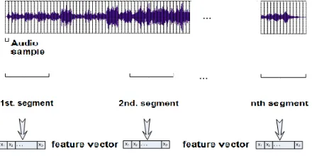
The music signal is naturally a time varying signal.Time decomposition is obtained considering feature vectors
ex-tracted from three 30-second segments (equivalent to 1,153 frames in a MP3 file) from the beginning, middle and end parts of the original music. We argue that this procedure is adequate for the problem, since it can better treat the time variation that is usual in music pieces. Also, it allows us to evaluate if the features extracted from different parts of the music have similar discriminative power. Figure 1 illustrate this process.
Figure 1. Time Decomposition Approach
2.2
Space decomposition
Despite being music genre classification naturally a multi-class problem, we accomplish the task using a com-bination of binary classifiers, whose results are merged in order to produce the final music genre labeling. Since dif-ferent features are used for difdif-ferent classes, the procedure characterize a space decomposition of the feature space, justified because in this case the classifiers tend to be sim-ple and effective [12]. Two main techniques are employed: (a) in the one-against-all (OAA) approach, a classifier is constructed for each class, and all the examples in the re-maining classes are considered as negative examples of that class; (b) in the round-robin(RR) approach, a classifier is constructed for each pair of classes, and the examples be-longing to the other classes are discarded. Figures 2 and 3 illustrate these approaches.
For am-class problem (mmusic genres) several classi-fiers are generated:mclassifiers in OAA andm(m−1)/2
classifiers in RR. The output of these classifiers are com-bined according to a decision procedure in order to produce the final class label.
2.3
Feature set
Figure 2. One-Against-All Space Decomposi-tion Approach
Figure 3. Round-Robin Space Decomposition Approach
Timbral Texture and Pitch Related. The Beat-Related fea-tures (feafea-tures 1 to 6) include the relative amplitudes and the beats per minute. The Timbral Texture features (features 7 to 25) account for the means and variance of the spectral centroid, rolloff, flux, the time zero domain crossings, the first 5 Mel Frequency Cepstral coefficients and low energy. Pitch Related features (features 26 to 30) include the maxi-mum periods and amplitudes of the pitch peaks in the pitch histograms. We note that most of the features are calculated over time intervals.
A normalization procedure is applied, in order to homog-enize the input data for the classifiers: ifmaxV andminV are the maximum and minimum values that appears in all dataset for a given feature, a valueV is replaced bynewV using the equation
newV = (V −minV) (maxV −minV)
The final feature vector, outlined at Table 1, is 30 -dimensional (Beat: 6; Timbral Texture: 19; Pitch: 5). For a more detailed description of the features refer to [21] or [18].
Table 1. Feature vector description Feature # Description
1 Relative amplitude of the first histogram peak 2 Relative amplitude of the second histogram peak 3 Ratio between the amplitudes of the second peak
and the first peak
4 Period of the first peak in bpm 5 Period of the second peak in bpm 6 Overall histogram sum (beat strength) 7 Spectral centroid mean
8 Spectral rolloff mean 9 Spectral flow mean 10 Zero crossing rate mean
11 Standard deviation for spectral centroid 12 Standard deviation for spectral rolloff 13 Standard deviation for spectral flow 14 Standard deviation for zero crossing rate 15 Low energy
16 1 rt. MFCC mean 17 2 nd. MFCC mean 18 3 rd. MFCC mean 19 4 th. MFCC mean 20 5 th. MFCC mean
21 Standard deviation for 1 rt. MFCC 22 Standard deviation for 2 nd. MFCC 23 Standard deviation for 3 rd. MFCC 24 Standard deviation for 4 th. MFCC 25 Standard deviation for 5 th. MFCC
26 The overall sum of the histogram (pitch strength) 27 Period of the maximum peak of the
unfolded histogram
28 Amplitude of maximum peak of the folded histogram
29 Period of the maximum peak of the folded histogram
30 Pitch interval between the two most prominent peaks of the folded histogram
2.4
Classification, Combination and
Deci-sion
Standard machine learning algorithms were employed as individual component classifiers. Our approach is homoge-neous, that is, the very same classifier is employed in every music part. In this work we use the following algorithms: Decision Trees (J48), k-NN, Na¨ıve-Bayes (NB), a Multi-layer Perceptron Neural Network Classifier (MLP) with the backpropagation momentum algorithm, and a Support Vec-tor Machines (SVM) with pairwise classification [15]. All the experiments were conducted in a framework based on the WEKA Datamining Tool [22].
strategies works as follows: (1) one of the space decompo-sition approaches (RR or OAA) is applied to all three seg-ments of the time decomposition approach (i.e. beginning, middle and end); (2) a local decision considering the class of the individual segment is made based on the underlying space decomposition approach: the majority vote for the RR and rules based on thea posterioriprobability given by the specific classifier of each case for the OAA; (3) the decision concerning the final music genre of the song is made based on the majority vote of the predicted genres from the three individual segments.
3
Feature Selection
The task of feature selection (FS) consists in choosing a proper subset of original feature set, in order to reduce the preprocessing and classification steps, but maintaining the final classification accuracy [3], [5]. The FS methods are often classified in two groups: the filter approach and the wrapper approach [16]. In the filter approach the fea-ture selection process is carried out before the use of any recognition algorithm. In the wrapper approach the pattern recognition algorithm is used as a sub-routine of the system to evaluate the generated solutions.
We emphasize that our system employs several feature vectors, according to time and space decompositions. FS procedure is employed in time segment vectors, allowing us to compare the relative importance of the features according to their time origin.
Our FS procedure is based on the genetic algorithm paradigm. Individuals (chromosomes) are n-dimensional binary vectors, wherenis the max feature vector size (30
in our case). Fitness of the individuals are obtained from the classification accuracy of the corresponding classifier, according to the wrapper approach.
The global feature selection procedure is as follows: 1. each individual works as a binary mask for an
associ-ated feature vector;
2. an initial assignment is randomly generated: a value1
indicates that the corresponding feature is used,0that it must be discarded;
3. a classifier is trained using the selected features; 4. the generated classification structure is applied to a
val-idation set to determine its accuracy, which is consid-ered as the fitness value of this individual;
5. we proceed elitism to conserve the top ranked individ-uals; crossover and mutation operators are applied in order to obtain the next generation.
In our FS procedure we employ 50 individuals in each generation, and the evolution process ends when it con-verges (no significant change in successive generations) or when a fixed max number of generations is achieved.
4
Experiments
This section presents the experiments and the results achieved on music genre classification and feature selection. The main goal is to evaluate if the features extracted from different origins in the audio signal have similar discrimi-native power for music genre classification. Another goal is to verify if the ensemble-based method provides better results than the classifiers taking into account features ex-tracted from single segments.
We employ the new Latin Music Database 1 [19], [18] which contains 3,227 MP3 music pieces from10different Latin genres, originated from music pieces of501artists. In this database music genre assignment was manually made by a group of human experts, based on the human per-ception of how each music is danced. The genre labeling was performed by two professional teachers with over 10 years of experience in teaching ballroom Latin and Brazil-ian dances.
The experiments were carried out on stratified training, validation and test datasets. In order to deal with balanced classes, three hundred different song tracks from each genre were randomly selected.
Our primary evaluation measure is the classification ac-curacy. Experiments were carry out using a ten-fold cross-validation procedure, that is, the presented results are ob-tained from 10 randomly independent experiment repeti-tions.
In Table 2 we present the results obtained with the ap-plication of the different classifiers to the beginning music segment (first 30 seconds). Since we are evaluating the fea-ture selection procedures using the MARSYAS framework, it is important to measure its performance without the use of any FS mechanism; this evaluation corresponds to the base-line (BL) presented in the second column. Columns 3 and 4 show the results for OAA and RR space decomposition approaches without feature selection; columns FS, FSOAA and FSRR show the corresponding results with the feature selection procedure. Results for the middle and end seg-ments can be found in [18].
Analogously, Table 3 presents global results using time and space decompositions, for OAA and RR approaches, with and without feature selection. We emphasize that this table encompasses the three time segments (beginning, mid-dle and end).
Summarizing the results in Table 3, we conclude that the FSRR method improves classification accuracy for the clas-sifiers J48, 3-NN and NB. Also, OAA and FSOAA methods present similar results for the MLP classifier, and only for the SVM classifier the best result is obtained without FS.
As previously mentioned, we also want to analyze if dif-ferent features have the same importance according to their
Table 2. Classification accuracy (%) using space decomposition for the beginning seg-ment of the music
Classifier BL OAA RR FS FSOAA FSRR
J48 39.60 41.56 45.96 44.70 43.52 48.53
3-NN 45.83 45.83 45.83 51.19 51.73 53.36
MLP 53.96 52.53 55.06 52.73 53.99 54.13 NB 44.43 42.76 44.43 45.43 43.46 45.39
SVM – 23.63 57.43 – 26.16 57.13
Table 3. Classification accuracy (%) using global time and space decomposition
Classifier BL OAA RR FS FSOAA FSRR
J48 47.33 49.63 54.06 50.10 50.03 55.46
3-NN 60.46 59.96 61.12 63.20 62.77 64.10
MLP 59.43 61.03 59.79 59.30 60.96 56.86 NB 46.03 43.43 47.19 47.10 44.96 49.79
SVM – 30.79 65.06 – 29.47 63.03
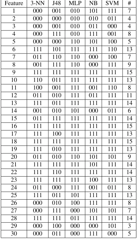
time origin. Table 4 shows a schematic map indicating the features selected in each time segment. In this table we em-ploy a binary BME mask – for (B)eginning, (M)iddle and (E)nd time segments – where 0 indicates that the feature was not selected and1indicated that it was selected by the FS procedure in the corresponding time segment.
In order to evaluate the discriminative power of the fea-tures, the last column in this table indicates how many times the corresponding feature was selected in the experiments (max 15 selections). Although this evaluation can be crit-icized, since different features can have different impor-tance according to the employed classifier, we argue that this counting gives an idea of the global feature discrimina-tive power. For example, features 6, 9, 10, 13, 15, 16, 17, 18, 13, 21, 22, 23, 25 and 28 are important for music genre classification. We remember that features 1 to 6 are Beat related, 7 to 25 are related to Timbral Texture, and 26 to 30 are Pitch related2.
5
Concluding Remarks
In this paper we evaluate a feature selection procedure based on genetic algorithms in the automatic music genre classification task. We also use an ensemble approach ac-cording to time and space decompositions: feature vectors
2See MARSYAS [21] for a complete description of the features.
Table 4. Selected features in each time seg-ment (BME mask)
Feature 3-NN J48 MLP NB SVM #
1 000 001 010 101 111 7
2 000 000 010 010 011 4
3 000 001 010 011 000 4
4 000 111 010 111 001 8
5 000 000 110 101 100 5
6 111 101 111 111 110 13
7 011 110 110 000 100 7
8 001 111 110 000 111 9
9 111 111 111 111 111 15
10 110 011 111 111 111 13
11 100 001 111 001 110 8
12 011 010 111 011 111 11 13 111 011 111 111 111 14
14 001 010 101 000 011 6
15 011 111 111 111 111 14 16 111 111 111 111 111 15 17 111 100 111 111 111 13 18 111 111 111 111 111 15 19 111 010 111 111 111 13
20 011 010 110 101 101 9
21 111 111 111 101 111 14 22 111 110 111 111 111 14 23 111 111 111 100 111 13
24 011 000 111 001 011 8
25 111 011 101 111 111 13
26 000 010 100 111 111 8
27 000 111 000 101 101 7
28 111 111 011 111 111 14
29 000 100 000 000 101 3
30 000 011 000 111 000 5
are selected from different time segments of the music, and one-against-all and round-robin composition schemes are employed for space decomposition. From the partial classi-fication results originated from these views, an unique final classification label is provided. We employ a large brand of classifiers and heuristic combination procedures in order to produce the final music genre label.
Experiments were conducted in a new large database – the Latin Music Database, with more than 3,000 music pieces from 10 music genres – methodically constructed for this research project [19], [18].
The results achieved with the feature selection show that this procedure is effective for J48, k-NN and Na¨ıve-Bayes classifiers; for MLP and SVM the FS procedure does not increases classification accuracy (Tables 2 and 3); these re-sults are compatible with the ones presented in [23].
We emphasize that the use of the time/space decompo-sition approach represents an interesting trade-off between classification accuracy and computational effort; also, the use of a reduced set of features implies a smaller processing time. This point is an important issue in practical applica-tions, where an adequate compromise between the quality of a solution and the time to obtain it must be achieved.
Another conclusion that can inferred from the experi-ments is that the features have different importance in the classification, according to their origin music segment (Ta-ble 4). It can be seen, however, that some features are present in almost every selection, showing they have a strong discriminative power in the classification task.
Indeed, the origin, number and duration of the time seg-ments, the use of space decomposition strategies and the definition of the more discriminative features still remain open questions for the automatic music genre classification problem.
References
[1] J. J. Aucouturier and F. Pachet. Representing musical genre: A state of the art.Journal of New Music Research, 32(1):83– 93, 2003.
[2] J. Bergstra, N. Casagrande, D. Erhan, D. Eck, and B. K´egl. Aggregate features and adaboost for music classification.
Machine Learning, 65(2-3):473–484, 2006.
[3] A. Blum and P. Langley. Selection of relevant features and examples in machine learning. Artificial Intelligence, 97(1-2):245–271, 1997.
[4] C. H. L. Costa, J. D. ValleJr, and A. L. Koerich. Automatic classification of audio data. InIEEE Intern. Conf. on Sys-tems, Man, and Cybernetics, pages 562–567, The Hague, Holand, 2004.
[5] M. Dash and H. Liu. Feature selection for classification.
Intelligent Data Analysis, 1(1–4):131–156, 1997.
[6] J. Downie and S. Cunningham. Toward a theory of music in-formation retrieval queries: System design implications. In
Proceedings of the 3rd Intern. Conf. on Music Information Retrieval, pages 299–300, 2002.
[7] R. Fiebrink and I. Fujinaga. Feature selection pitfalls and music classification. In Proc. of the 7th Intern. Conf. on Music Information Retrieval, pages 340–341, Victoria, CA, 2006.
[8] M. Grimaldi, P. Cunningham, and A. Kokaram. A wavelet packet representation of audio signals for music genre clas-sification using different ensemble and feature selection
techniques. InProc. of the 5th ACM SIGMM Intern. Work-shop on Multimedia Information Retrieval, pages 102–108, 2003.
[9] J. Lee and J. Downie. Survey of music information needs, uses, and seeking behaviours: preliminary findings. InProc. of the 5th Intern. Conf. on Music Information Retrieval, pages 441–446, Barcelona, Spain, 2004.
[10] M. Li and R. Sleep. Genre classification via an lz78-based string kernel. InProc. of the 6th Intern. Conf. on Music Information Retrieval, pages 252–259, London, UK, 2005. [11] T. Li and M. Ogihara. Music genre classification with
tax-onomy. InProc. of IEEE Intern. Conf. on Acoustics, Speech and Signal Processing, pages 197–200, Philadelphia, USA, 2005.
[12] H. Liu and L. Yu. The Handbook of Data Mining, chapter Feature Extraction, Selection, and Construction, pages 409– 424. Lawrence Erlbaum Publishers, 2003.
[13] C. McKay and I. Fujinaga. Musical genre classification: Is it worth pursuing and how can it be? InProc. of the 7th Intern. Conf. on Music Information Retrieval, pages 101– 106, Victoria, CA, 2006.
[14] A. Meng, P. Ahrendt, and J. Larsen. Improving music genre classification by short-time feature integration. InIEEE In-tern. Conf. on Acoustics, Speech, and Signal Processing, pages 497–500, Philadelphia, PA, USA, 2005.
[15] T. M. Mitchell.Machine Learning. McGraw-Hill, 1997. [16] L. Molina, L. Belanche, and A. Nebot. Feature selection
algorithms: a survey and experimental evaluation. InProc. of the IEEE Intern. Conf. on Data Mining, pages 306–313, Maebashi City, JP, 2002.
[17] C. Silla Jr., C. Kaestner, and A. L. Koerich. Automatic mu-sic genre classification using ensemble of classifiers (in por-tuguese). InProc. of the IEEE International Conference on Systems, Man and Cybernetics (SMC 2007), pages 1687– 1692, Montreal, Canada, 2007.
[18] C. N. Silla Jr.Classifiers Combination for Automatic Music Classification (in portuguese). MSc dissertation, Graduate Program in Applied Computer Science, Pontifical Catholic University of Paran´a, 2007.
[19] C. N. Silla Jr., A. L. Koerich, and C. A. A. Kaestner. The latin music database. InProceedings of the 9th International Conference on Music Information Retrieval, pages 451–456, 2008.
[20] C. SillaJr., C. Kaestner, and A. L. Koerich. Time-space ensemble strategies for automatic music genre classifica-tion. InBrazilian Symposium on Artificial Intelligence (Lec-ture Notes in Computer Science, Vol.4140), pages 339–348, 2006.
[21] G. Tzanetakis and P. Cook. Musical genre classification of audio signals.IEEE Transactions on Speech and Audio Pro-cessing, 10(5):293–302, 2002.
[22] I. H. Witten and E. Frank. Data Mining: Practical ma-chine learning tools and techniques. Morgan Kaufmann, San Francisco, 2nd edition, 2005.